Code
library(banditsCI)
library(ggplot2)
library(dplyr)
library(tidyr)

set.seed(123)If you have ever:
…welcome. You are among friends.
Contextual bandits are the caffeinated cousin of A/B testing: they learn who should get what while the experiment is running. That is fantastic for product outcomes—you waste fewer impressions on the losing variant and can tailor treatment to user segments on the fly. But it makes inference awkward. Standard tools (t-tests, naive regression, difference-in-means) tend to act overconfident when the data were collected adaptively, because the assignment mechanism itself evolves with the outcomes it has already seen.
The core tension is this: a bandit algorithm uses past outcomes to decide future assignments. That feedback loop means observations are no longer independent draws from a fixed assignment rule, which is the assumption behind most of the inference machinery we learned in our first econometrics course. You can still get a reasonable point estimate from bandit-collected data, but the standard errors and confidence intervals that come out of off-the-shelf tools will generally be wrong—and wrong in the dangerous direction (too narrow).
In this tutorial we build a full, reproducible workflow in R using the banditsCI package (Offer-Westort and Zhou 2024), which implements frequentist inference for adaptively generated data based on the methods in Hadad et al. and Zhan et al. (Hadad et al. 2021; Zhan et al. 2021). We will also connect the practical recipe to more recent theory on post-contextual-bandit inference (Bibaut et al. 2021) and newer work on when classical tests have non-Gaussian limits unless the sampling scheme satisfies additional structure (Akker, Werker, and Zhou 2025).
Who is this for? You should be comfortable with R, familiar with the basics of A/B testing, and have at least passing familiarity with concepts like inverse propensity weighting. If you have ever thought about heterogeneous treatment effects or policy learning, even better—but it is not a prerequisite.
High-level roadmap. We are going to separate two distinct jobs:
If you blend these two jobs carelessly—for instance, by using the same model for both allocation and evaluation without proper debiasing—the algorithm may still “work” in terms of maximizing reward, but your confidence intervals will not cover at the advertised rate.
Think of a very common marketing/UX scenario:
X consisting of a few stable user segments and behavioral covariates.W ∈ {1, 2} and observe a reward Y (conversion, click, revenue).In a standard A/B test, you would assign variants uniformly at random, wait until the experiment ends, and then run a test. That is clean, but it also means you keep showing the worse variant to users even after the data strongly suggest it is inferior. A contextual bandit tries to learn which variant works better for which types of users while the experiment is running, shifting traffic toward the better-performing arm as evidence accumulates. The price of that efficiency is that inference becomes harder.
We will simulate everything end-to-end so we always know the truth and can check whether our inference pipeline recovers it.
library(banditsCI)
library(ggplot2)
library(dplyr)
library(tidyr)
set.seed(123)One small helper function before we begin. The ridge_muhat_lfo_pai() function in banditsCI returns a 3D array of conditional mean estimates. We need to extract the diagonal slice that corresponds to “the model’s prediction for time \(t\), using only data available up to time \(t\)” (the leave-future-out structure). This is exactly what the package vignette does (banditsCI package authors 2024), and the function below handles that extraction:
diag_slice_mu_hat <- function(mu_hat_3d) {
  mu2 <- mu_hat_3d[1,,]
  for (i in seq_len(nrow(mu2))) mu2[i,] <- mu_hat_3d[i, i,]
  mu2
}Before we can stress-test any inference method, we need a world where we actually know the answer. Simulation gives us that. We’re going to generate two objects:
xs: a matrix of contexts with shape [A, p], where A is the number of time steps (users) and p is the number of context features.ys: a matrix of potential outcomes with shape [A, K], where ys[t, w] is what we would observe if we assigned arm w at time t.The potential outcomes framework is doing important conceptual work here. In real life, you only ever observe one outcome per user: yobs[t] = ys[t, ws[t]], where ws[t] is what the bandit chose. The other potential outcome is counterfactual. In simulation, we get to see both—so we can compute the true value of any policy and check whether our intervals behave.
If you’ve ever looked at conversion or revenue data and thought “wow, this is… not very Gaussian,” you’re right. Two features show up constantly in product/marketing metrics:
To make the tutorial more honest—and to give the weighting schemes something real to do—we’ll let the noise scale depend on context. Concretely, users with large (|X_1|) will have noisier outcomes. We’ll also include an optional switch for heavier-tailed noise.
make_linear_bandit_data <- function(A = 5000, K = 2, p = 6,
                                   noise_sd = 1.0,
                                   heteroskedastic = TRUE,
                                   heavy_tails = FALSE,
                                   df_t = 3) {
  stopifnot(K == 2)  # keep the tutorial tight; extension to K>2 is in the appendix
  xs <- matrix(rnorm(A * p), ncol = p)

  # True linear reward model with treatment effect heterogeneity:
  # Arm 1 tends to win when X1 > 0; arm 2 wins when X1 < 0.
  # Both arms share the same X2 coefficient, so X2 shifts the level but
  # doesn't change which arm is better.
  beta1 <- c(+0.7, 0.25, rep(0, p - 2))
  beta2 <- c(-0.7, 0.25, rep(0, p - 2))

  mu1 <- as.numeric(xs %*% beta1)
  mu2 <- as.numeric(xs %*% beta2)

  # --- Noise model ---
  # Heteroskedastic: users with more extreme X1 are noisier (common in practice).
  # This keeps the mean structure unchanged but makes inference harder in a realistic way.
  if (heteroskedastic) {
    sd_t <- noise_sd * (0.5 + 1.5 * abs(xs[, 1]))  # always positive
  } else {
    sd_t <- rep(noise_sd, A)
  }

  # Optionally use heavy-tailed noise (Student-t) instead of Gaussian.
  # Useful if you want to mimic revenue-ish metrics with occasional outliers.
  if (heavy_tails) {
    eps1 <- rt(A, df = df_t) * sd_t
    eps2 <- rt(A, df = df_t) * sd_t
  } else {
    eps1 <- rnorm(A, sd = sd_t)
    eps2 <- rnorm(A, sd = sd_t)
  }

  ys <- cbind(mu1 + eps1, mu2 + eps2)

  muxs <- cbind(mu1, mu2)  # conditional mean reward per arm (truth, without noise)
  best_arm <- ifelse(mu1 >= mu2, 1L, 2L)

  list(xs = xs, ys = ys, muxs = muxs, best_arm = best_arm, A = A, K = K, p = p, sd_t = sd_t)
}

data <- make_linear_bandit_data(
  A = 5000, K = 2, p = 6,
  noise_sd = 1.0,
  heteroskedastic = TRUE,
  heavy_tails = FALSE
)

xs <- data$xs
ys <- data$ys
A  <- data$A
K  <- data$K
A few things to note about this data-generating process. The average treatment effect is heterogeneous and it is driven almost entirely by the first context variable: when (X_1 > 0), arm 1 has higher expected reward; when (X_1 < 0), arm 2 does. The second feature (X_2) shifts both arms up and down together, so it affects the level of outcomes but not which arm is optimal. The remaining covariates are mostly noise—useful as “distractors” that make the learning problem feel more like real telemetry.
Another (optional) component is the noise structure. Outcomes are heteroskedastic: some contexts are simply noisier than others (here, extreme values of (|X_1|) generate higher variance). If you turn on the heavy-tail option, you also get occasional outliers. This doesn’t change which arm is better on average, but it absolutely changes how hard it is to get well-calibrated uncertainty out of adaptive data. In other words, the bandit still has something clean to learn, but the inference problem is now closer to what we see in practice.
Since we know the true conditional means muxs, we can define an oracle policy: always pick the arm with the larger expected reward for each user’s context. This is the best any policy could do if it had perfect knowledge of the data-generating process. We use it as our ground truth yardstick for evaluating inference quality.
policy_oracle <- matrix(0, nrow = A, ncol = K)
policy_oracle[cbind(seq_len(A), data$best_arm)] <- 1

truth_oracle_value <- mean(ys[cbind(seq_len(A), data$best_arm)])
truth_oracle_value
[1] 0.5167168Now we let a bandit algorithm allocate arms. banditsCI implements Linear Thompson Sampling, which works as follows at each time step: maintain a Bayesian linear model of reward as a function of context for each arm, draw a sample from each arm’s posterior, and assign the user to the arm whose sampled reward is highest. Early on, the posteriors are wide and the algorithm explores broadly. As data accumulates, the posteriors tighten and the algorithm increasingly exploits what it has learned.
A key practical knob is the probability floor. In principle, Thompson Sampling can assign a near-zero probability to an arm it has become very confident about. That is great for regret minimization, but it causes serious problems for inference: the importance weights (inverse of assignment probability) explode, and variance blows up. A probability floor constrains the minimum assignment probability to stay above some threshold. Think of it as a seatbelt: slightly uncomfortable in normal driving, but you will appreciate it when something goes wrong. Setting floor_start = 0.005 means no arm’s assignment probability can drop below 0.5%.
batch_sizes <- rep(1000, 5)

results <- run_experiment(
  ys = ys,
  xs = xs,
  floor_start = 0.005,
  floor_decay = 0,
  batch_sizes = batch_sizes
)

str(results[c("ws", "yobs", "probs")])
List of 3
$ ws : num [1:5000] 1 2 1 2 1 1 2 1 2 2 ...
$ yobs : num [1:5000] -0.775 0.748 -0.723 -0.129 0.945 ...
$ probs: num [1:5000, 1:5000, 1:2] 0.5 0.5 0.5 0.5 0.5 0.5 0.5 0.5 0.5 0.5 ...The batch_sizes argument controls how often the bandit updates its model. Here we use five batches of 1,000 observations each, meaning the bandit re-estimates its reward model after every 1,000 users. In practice, batch sizes are often dictated by operational constraints (how often can you update your serving model?) and inferential considerations (larger batches mean fewer adaptation points, which can simplify the asymptotic arguments).
Let’s start with a cumulative assignment plot to see whether the algorithm shifted traffic over time:
plot_cumulative_assignment(results, batch_sizes)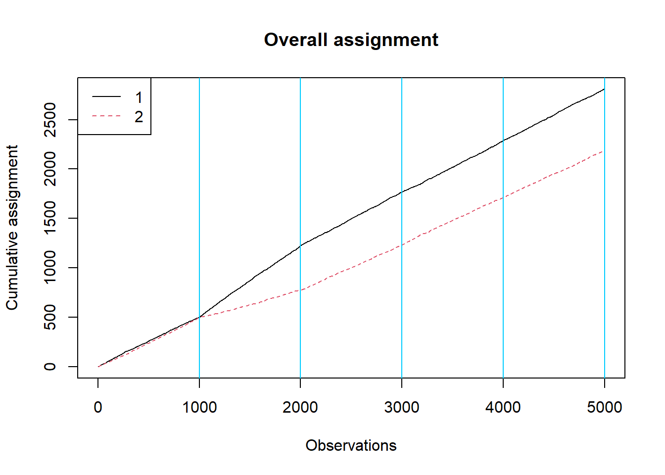
And a more targeted diagnostic: within each true best-arm group, how often does the bandit assign the correct arm? If the algorithm is learning the context-reward relationship, we should see this probability increase over time.
df_assign <- tibble(
  t = seq_len(A),
  best = data$best_arm,
  chosen = results$ws
)

ggplot(df_assign, aes(x = t, y = as.integer(chosen == best))) +
  geom_smooth(se = FALSE, span = 0.2) +
  labs(
    title = "Did the bandit learn context?",
    subtitle = "Rolling probability of choosing the true best arm",
    x = "time (t)",
    y = "Pr(chosen arm = true best arm)"
  )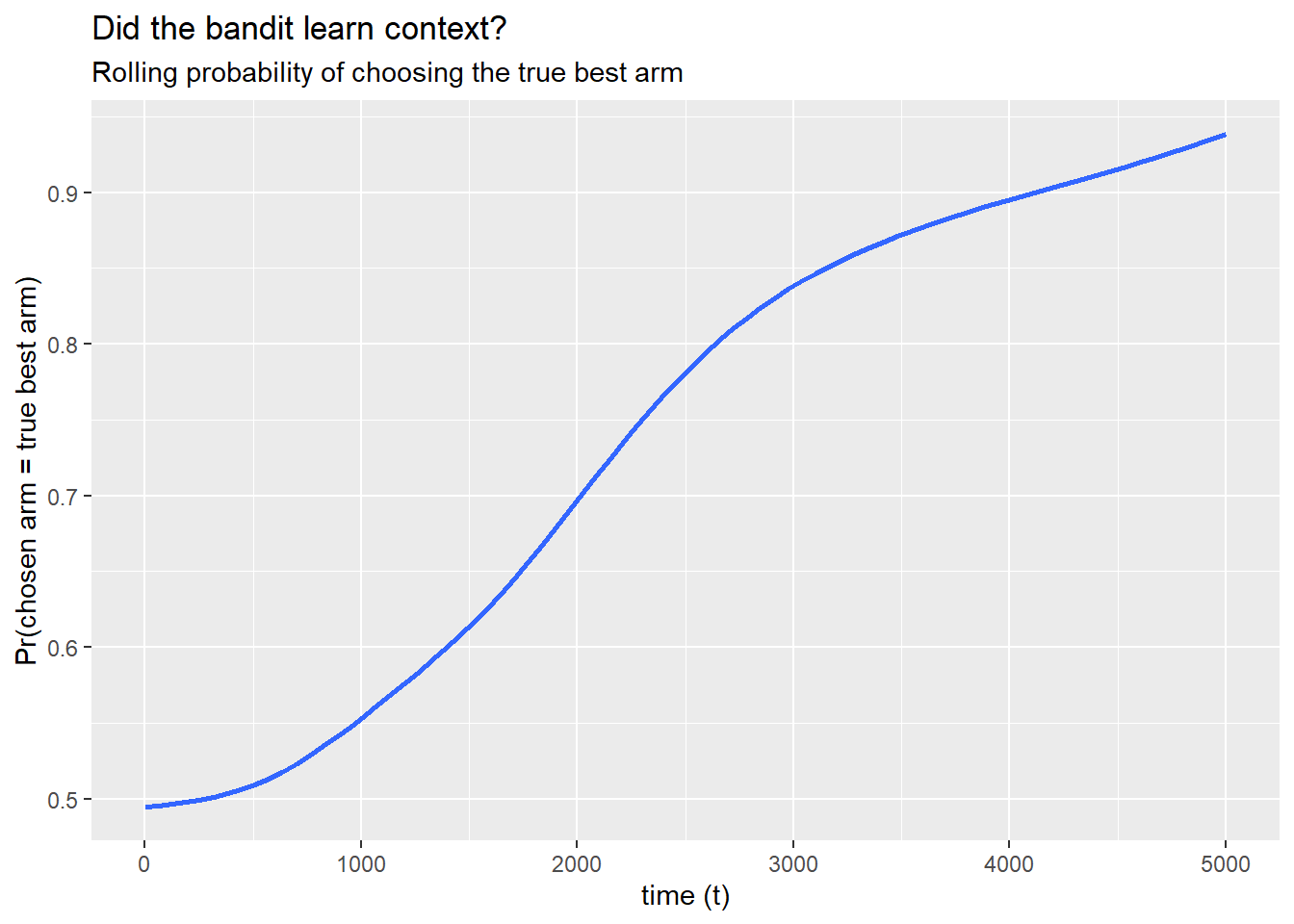
If this line trends upward from around 0.5 (random guessing) toward 0.7 or higher, the bandit is doing its job: it is learning which arm to serve based on the user’s context.
The bandit returns results$probs[t, w] = \(\Pr(W_t = w \mid \text{history}, X_t)\) for every arm at every time step.
For inference, the critical quantity is the probability of the arm actually chosen at each time step. This is what enters the inverse propensity weight. If many of these probabilities are close to zero, the IPW weights will be huge and inference will be unstable—regardless of what fancy weighting scheme you use downstream. This is why we set a floor.
p_chosen <- results$probs[cbind(seq_len(A), results$ws)]

ggplot(tibble(p = p_chosen), aes(x = p)) +
  geom_histogram(bins = 40) +
  labs(
    title = "Logged assignment probabilities for chosen arms",
    subtitle = "If this piles up near 0, your IPW weights will get spicy",
    x = "P(W_t = chosen | history, X_t)",
    y = "count"
  )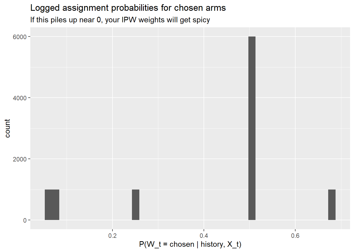
What you want to see: a distribution that stays well above zero with most of the mass between, say, 0.3 and 0.9. What you do not want: a spike near 0 or 1. A spike near 0 means the algorithm is making confident assignments that happened to go the other way (rare events with huge weights). A spike near 1 means the algorithm has essentially converged and is barely exploring—good for regret, tricky for inference.
Let’s pretend, for a moment, that we forgot the data were adaptively collected. We just compute a plain difference in sample means between the two arms:
naive_diff <- mean(results$yobs[results$ws == 2]) - mean(results$yobs[results$ws == 1])
naive_diff
[1] 0.01239785This number is not automatically garbage. The point estimate might even be in the right ballpark. The problem is the uncertainty quantification that people typically attach to it. A standard \(t\)-test or OLS standard error assumes that treatment assignment is independent of potential outcomes conditional on covariates. Under adaptive assignment, that assumption fails in a specific way:
The upshot: you might get a reasonable point estimate paired with a wildly overconfident standard error. That is the dangerous combination—it makes you think you know more than you do.
So instead of naive estimation, we do policy evaluation the way banditsCI intends.
This is the core of the inferential workflow. The goal is to estimate the value of a given policy—“if we deployed this rule for assigning arms to users, what average reward would we expect?”—and to get valid confidence intervals for that estimate, despite the data having been collected adaptively.
The approach has two main ingredients, and it is worth understanding why we need both.
The first ingredient is a doubly robust (or augmented inverse propensity weighted, AIPW) score for each observation. The intuition is as follows. We have two sources of information about what would have happened under a different assignment policy:
Either source alone has a weakness. The outcome model can be misspecified. The propensity weights can have high variance (especially when probabilities are near zero). The AIPW score combines both: it starts from the outcome model’s prediction and adds a bias correction term based on the propensity-weighted residual. The resulting estimator is doubly robust—it is consistent if either the outcome model or the propensity model is correctly specified.
The key subtlety in the bandit setting is that the outcome model \(\hat{\mu}_t\) must be fit using only data available at or before time \(t\). If you fit a single model on all the data and then use it to compute scores, you are leaking future information into the score construction, which invalidates the inference. The banditsCI package enforces this through a leave-future-out (batch-wise) ridge regression via ridge_muhat_lfo_pai() (banditsCI package authors 2024).
mu_hat_3d <- ridge_muhat_lfo_pai(
  xs = xs,
  ws = results$ws,
  yobs = results$yobs,
  K = K,
  batch_sizes = batch_sizes
)

mu_hat <- diag_slice_mu_hat(mu_hat_3d)
The second piece is the adaptive weighting. Under uniform (i.i.d.) data collection, you would weight every observation equally. Under adaptive collection, observations from early time periods (when the algorithm was still exploring) are more informative for inference than observations from later periods (when the algorithm has largely converged). The calculate_balwts() function computes weights that account for this:
balwts <- calculate_balwts(results$ws, results$probs)Now we can assemble the AIPW scores:
aipw_scores <- aw_scores(
  ws = results$ws,
  yobs = results$yobs,
  mu_hat = mu_hat,
  K = K,
  balwts = balwts
)With the AIPW scores in hand, we can evaluate any policy we like. A “policy” is represented as an [A, K] matrix where entry [t, w] is the probability that the policy assigns arm w to the user at time t. Deterministic policies have entries that are 0 or 1.
policy_arm1 <- matrix(0, nrow = A, ncol = K); policy_arm1[, 1] <- 1
policy_arm2 <- matrix(0, nrow = A, ncol = K); policy_arm2[, 2] <- 1
Now we evaluate each policy under three weighting schemes:
uniform: weights all observations equally. This is the default in most applied work, but it can be overly optimistic under adaptivity because it does not account for the changing assignment probabilities.contextual_minvar: minimizes the estimated variance of the policy value estimator, taking the contextual (covariate-dependent) structure into account.contextual_stablevar: a stabilized variant that trades a small amount of efficiency for better finite-sample robustness. This is often the most reliable choice in practice.These correspond to the methods proposed in Hadad et al. and Zhan et al. (Hadad et al. 2021; Zhan et al. 2021).
eval_policies <- function(policy_list) {
  output_estimates(
    policy1 = policy_list,
    gammahat = aipw_scores,
    probs_array = results$probs,
    floor_decay = 0,
    uniform = TRUE,
    contextual_minvar = TRUE,
    contextual_stablevar = TRUE,
    non_contextual_minvar = FALSE,
    non_contextual_stablevar = FALSE,
    non_contextual_twopoint = FALSE
  )
}

out <- eval_policies(list(policy_arm1, policy_arm2, policy_oracle))
names(out) <- c("Always arm 1", "Always arm 2", "Oracle policy")
Each element of out is a small table where rows are weighting schemes and columns include estimate and std.error. Let’s look at the oracle policy:
out[["Oracle policy"]] estimate std.error
uniform 0.5263514 0.03304980
non_contextual_minvar NA NA
contextual_minvar 0.5298095 0.03193969
non_contextual_stablevar NA NA
contextual_stablevar 0.5278543 0.03209141
non_contextual_twopoint NA NATo make comparisons easier, we’ll reshape everything into one data frame with confidence intervals:
tidy_out <- bind_rows(lapply(names(out), function(name) {
  tab <- as.data.frame(out[[name]])
  tab$scheme <- rownames(tab)
  tab$policy <- name
  tab
}), .id = NULL) %>%
  mutate(
    lower = estimate - 1.96 * std.error,
    upper = estimate + 1.96 * std.error
  )

tidy_out %>%
  select(policy, scheme, estimate, std.error, lower, upper) %>%
  arrange(policy, scheme)
policy scheme
contextual_minvar...1 Always arm 1 contextual_minvar
contextual_stablevar...2 Always arm 1 contextual_stablevar
non_contextual_minvar...3 Always arm 1 non_contextual_minvar
non_contextual_stablevar...4 Always arm 1 non_contextual_stablevar
non_contextual_twopoint...5 Always arm 1 non_contextual_twopoint
uniform...6 Always arm 1 uniform
contextual_minvar...7 Always arm 2 contextual_minvar
contextual_stablevar...8 Always arm 2 contextual_stablevar
non_contextual_minvar...9 Always arm 2 non_contextual_minvar
non_contextual_stablevar...10 Always arm 2 non_contextual_stablevar
non_contextual_twopoint...11 Always arm 2 non_contextual_twopoint
uniform...12 Always arm 2 uniform
contextual_minvar...13 Oracle policy contextual_minvar
contextual_stablevar...14 Oracle policy contextual_stablevar
non_contextual_minvar...15 Oracle policy non_contextual_minvar
non_contextual_stablevar...16 Oracle policy non_contextual_stablevar
non_contextual_twopoint...17 Oracle policy non_contextual_twopoint
uniform...18 Oracle policy uniform
estimate std.error lower upper
contextual_minvar...1 0.02591384 0.04752126 -0.06722782 0.11905551
contextual_stablevar...2 -0.05221602 0.07071204 -0.19081162 0.08637957
non_contextual_minvar...3 NA NA NA NA
non_contextual_stablevar...4 NA NA NA NA
non_contextual_twopoint...5 NA NA NA NA
uniform...6 -0.38530042 0.27211613 -0.91864802 0.14804719
contextual_minvar...7 -0.02699118 0.05271545 -0.13031347 0.07633110
contextual_stablevar...8 -0.02313075 0.05616767 -0.13321938 0.08695788
non_contextual_minvar...9 NA NA NA NA
non_contextual_stablevar...10 NA NA NA NA
non_contextual_twopoint...11 NA NA NA NA
uniform...12 0.03180494 0.07618343 -0.11751459 0.18112448
contextual_minvar...13 0.52980950 0.03193969 0.46720770 0.59241130
contextual_stablevar...14 0.52785434 0.03209141 0.46495518 0.59075350
non_contextual_minvar...15 NA NA NA NA
non_contextual_stablevar...16 NA NA NA NA
non_contextual_twopoint...17 NA NA NA NA
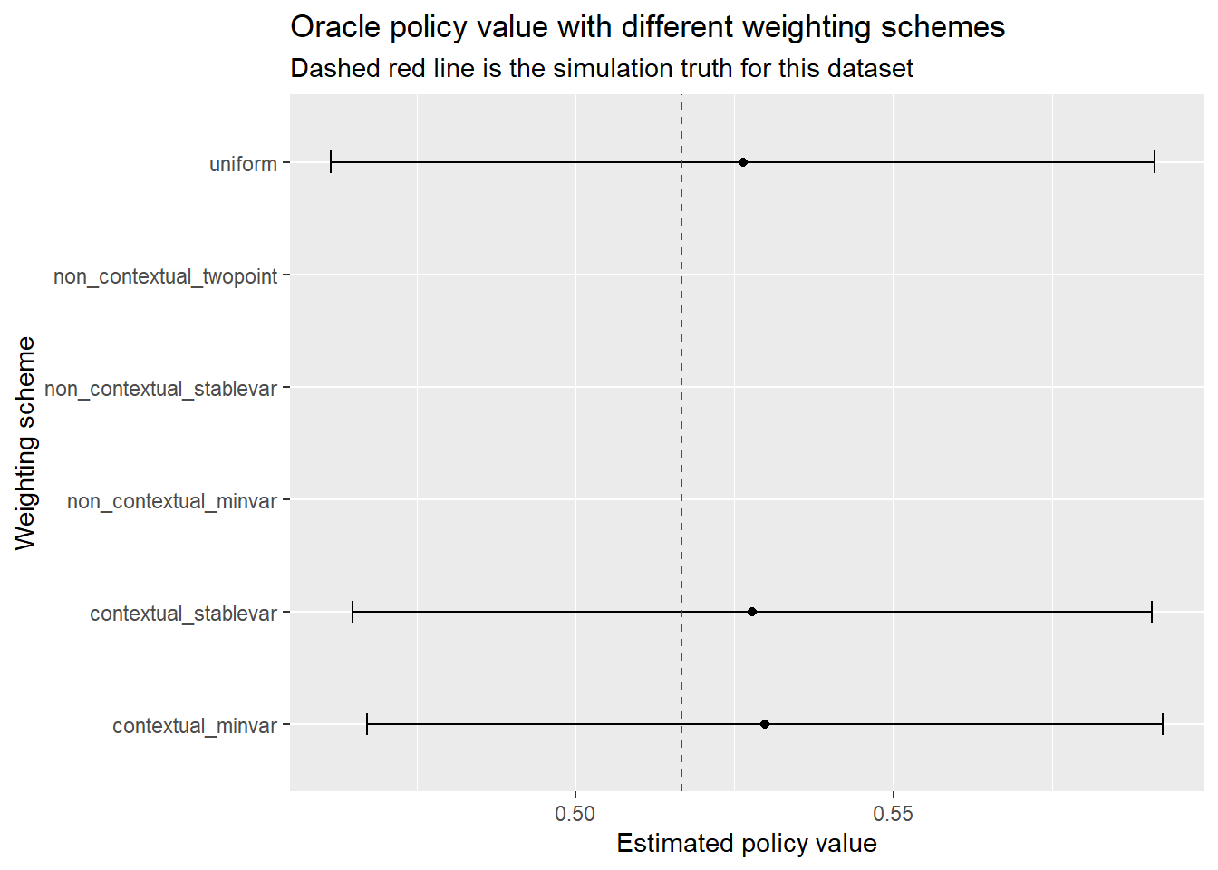
uniform...18 0.52635135 0.03304980 0.46157374 0.59112896A few things to look for in this table. First, do the confidence intervals for the oracle policy contain the true oracle value we computed earlier? Second, how do the interval widths compare across weighting schemes? If contextual_stablevar gives tighter intervals than uniform while maintaining coverage, that is the adaptive weighting earning its keep.
ggplot(
  tidy_out %>% filter(policy == "Oracle policy"),
  aes(x = estimate, y = scheme)
) +
  geom_point() +
  geom_errorbarh(aes(xmin = lower, xmax = upper), height = 0.2) +
  geom_vline(xintercept = truth_oracle_value, linetype = "dashed", color = "red") +
  labs(
    title = "Oracle policy value with different weighting schemes",
    subtitle = "Dashed red line is the simulation truth for this dataset",
    x = "Estimated policy value",
    y = "Weighting scheme"
  )
One simulation draw can be misleading. Maybe we got lucky. Maybe the bandit happened to explore in a pattern that made inference easy. The only way to know whether our confidence intervals are actually calibrated is to repeat the entire experiment many times and check.
Monte Carlo coverage works like this:
If the method is well-calibrated, coverage should be close to 95%. If it comes in at 60%, your “95% confidence interval” is actually a 60% confidence interval—which is to say, not very confidence-inspiring at all. This is particularly important in the bandit setting because, as we discussed, the adaptive assignment mechanism can cause standard methods to undercover.
A note on real deployments. You never know the ground truth in production. Monte Carlo coverage checks are how you validate your inference pipeline before deploying it. Think of it as a unit test for your statistical method: you run it in a controlled environment where you know the answer, and if it passes, you gain confidence that it will work in the wild.
We wrap the entire pipeline—data generation, bandit run, AIPW score construction, and policy evaluation—into a single function:
simulate_once <- function(seed, A = 3000, p = 6, noise_sd = 1.0,
                          floor_start = 0.005, batch_sizes = rep(600, 5)) {
  set.seed(seed)

  dat <- make_linear_bandit_data(A = A, K = 2, p = p, noise_sd = noise_sd)
  xs <- dat$xs
  ys <- dat$ys

  truth_oracle <- mean(ys[cbind(seq_len(A), dat$best_arm)])

  res <- run_experiment(
    ys = ys,
    xs = xs,
    floor_start = floor_start,
    floor_decay = 0,
    batch_sizes = batch_sizes
  )

  mu_hat_3d <- ridge_muhat_lfo_pai(
    xs = xs, ws = res$ws, yobs = res$yobs, K = 2, batch_sizes = batch_sizes
  )
  mu_hat <- diag_slice_mu_hat(mu_hat_3d)
  balwts <- calculate_balwts(res$ws, res$probs)

  aipw_scores <- aw_scores(ws = res$ws, yobs = res$yobs, mu_hat = mu_hat, K = 2, balwts = balwts)

  policy_oracle <- matrix(0, nrow = A, ncol = 2)
  policy_oracle[cbind(seq_len(A), dat$best_arm)] <- 1

  out <- output_estimates(
    policy1 = list(policy_oracle),
    gammahat = aipw_scores,
    probs_array = res$probs,
    floor_decay = 0,
    uniform = TRUE,
    contextual_minvar = TRUE,
    contextual_stablevar = TRUE,
    non_contextual_minvar = FALSE,
    non_contextual_stablevar = FALSE,
    non_contextual_twopoint = FALSE
  )[[1]]

  tab <- as.data.frame(out)
  tab$scheme <- rownames(tab)
  tab$truth <- truth_oracle
  tab$lower <- tab$estimate - 1.96 * tab$std.error
  tab$upper <- tab$estimate + 1.96 * tab$std.error
  tab$covered <- (tab$lower <= tab$truth) & (tab$truth <= tab$upper)

  tab
}Fifty replicates is enough to see broad patterns, though you would want more (say 500–1000) for a paper. The results will tell us which weighting schemes deliver on their coverage promise.
mc <- bind_rows(lapply(1:50, function(s) simulate_once(seed = 1000 + s)))
mc %>%
  group_by(scheme) %>%
  summarize(
    coverage = mean(covered),
    avg_width = mean(upper - lower),
    .groups = "drop"
  ) %>%
  arrange(desc(coverage))
# A tibble: 6 × 3
scheme coverage avg_width
<chr> <dbl> <dbl>
1 contextual_minvar 1 0.166
2 contextual_stablevar 1 0.169
3 uniform 1 0.178
4 non_contextual_minvar NA NA
5 non_contextual_stablevar NA NA
6 non_contextual_twopoint NA NA Two things to look for: coverage close to 0.95, and reasonable interval width. A method that achieves 95% coverage by producing absurdly wide intervals is technically valid but not very useful. The best method delivers coverage and short intervals.
mc_sum <- mc %>%
  group_by(scheme) %>%
  summarize(coverage = mean(covered), .groups = "drop")

ggplot(mc_sum, aes(x = scheme, y = coverage)) +
  geom_col() +
  geom_hline(yintercept = 0.95, linetype = "dashed", color = "red") +
  coord_cartesian(ylim = c(0, 1)) +
  labs(
    title = "Monte Carlo coverage of 95% CIs",
    subtitle = "Dashed red line = 0.95 (target coverage)",
    x = NULL,
    y = "Coverage"
  )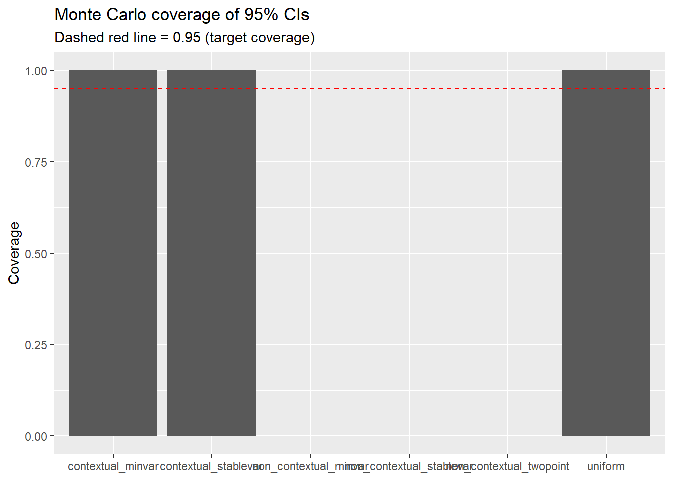
How to read this plot. If uniform undercovers (bar falls well below the red line) but contextual_stablevar stays close to 0.95, that is the entire “bandits need bandit-aware inference” message distilled into one picture. The uniform weighting scheme pretends the data were collected under a fixed design; the adaptive schemes know better.
Even if you never open any of the theory papers referenced here, following this checklist will help you avoid most of the common pitfalls.
You cannot do valid post-hoc inference on bandit data if you did not log the right things. At minimum:
Two developments at the frontier that are worth knowing about, especially if you are thinking about deploying contextual bandits at scale:
CADR (Contextual Adaptive Doubly Robust) estimation (Bibaut et al. 2021) provides a framework for constructing asymptotically normal policy value estimators under contextual adaptive data collection. The key insight is that the standard martingale CLT arguments used in the non-contextual case need to be augmented with a careful treatment of how the context distribution interacts with the adaptive assignment rule. This gives practitioners a principled way to build confidence intervals that remain valid even when the bandit conditions on high-dimensional contexts.
Non-Gaussian limits for classical tests (Akker, Werker, and Zhou 2025). This is a cautionary result: it shows that standard \(t\)-tests and IPW-based test statistics can have non-Gaussian asymptotic distributions under adaptive data collection, unless the sampling scheme satisfies a structural condition called translation invariance. The paper also proposes translation-invariant variants of common bandit algorithms that restore Gaussian limits. The practical takeaway is that the algorithm you choose is not just an engineering decision—it is part of the data-generating process and directly affects what inference methods are valid downstream.
Together, these results reinforce a single message: in the bandit setting, design and analysis are not separable. The choices you make about how to allocate arms constrain what you can credibly say afterward. This is a departure from the classical experimental design mindset, where the randomization scheme is fixed and the analyst’s job is purely post-hoc. In bandits, the analyst needs to be in the room when the allocation rule is being designed.
This post uses K = 2 to keep the narrative and visuals manageable. Everything here generalizes directly to K > 2 with the same banditsCI workflow. The main changes are:
[A, K] with the appropriate number of columns.K separate arm-level estimates that are hard to interpret jointly.The simplest way to experiment: change K = 4 in make_linear_bandit_data(), define distinct coefficient vectors for each arm, and construct the oracle policy using apply(muxs, 1, which.max).