How to estimate causal effects with unmeasured confounding using proxy variables, with a worked simulation and a real-data walkthrough in R.
Author
Felicia Nguyen
Published
November 18, 2025
Why I care about proximal causal inference
Most of the causal estimators I reach for day-to-day—regression adjustment, matching, inverse probability weighting, doubly robust estimators—lean heavily on a version of conditional exchangeability (a.k.a. “selection on observables” or “no unmeasured confounding”):
\[
Y(a) \perp\!\!\!\perp A \mid X
\]
where \(A\) is the treatment, \(Y\) is the outcome, \(X\) are measured covariates, and \(Y(a)\) is the potential outcome under treatment level \(a\).
The problem is that in a lot of the observational work I care about, I don’t fully buy \(Y(a) \perp\!\!\!\perp A \mid X\). Sometimes the missing piece is a substantively important confounder \(U\) that is hard (or impossible) to measure well: ability, motivation, latent health status, risk preference, clinician judgment, seller quality, algorithmic recommendation intensity, etc. We’ve all been in that seminar where someone raises their hand and says “but what about unobserved heterogeneity?”—and the presenter takes a long sip of water.
Proximal causal inference (PCI) is one of the cleanest frameworks I know for making progress in exactly that setting: unmeasured confounding exists, but we have proxy variables that carry information about the unmeasured confounder(s). The canonical identification results trace back to proxy-variable work in Biometrika and were later organized into a “proximal g-formula” framework (Miao, Geng, and Tchetgen Tchetgen 2018; Tchetgen Tchetgen et al. 2024). The basic idea has been around for a while, but there’s been an explosion of methodological work in the last few years, including extensions to survival data, mediation, time-varying treatments, and semiparametric estimation (Cui et al. 2024; Liu et al. 2025; Ringlein et al. 2025).
This post is my attempt to give a working, applied introduction:
The setup and the assumptions (in plain language).
The “bridge function” trick that makes identification work.
A full implementation in R:
a simulation where we know the truth,
a real-data illustration using the wage2 dataset.
Practical tips, diagnostics, and failure modes.
I’ll keep the discussion at the “what I need to run this responsibly” level, and I’ll flag where things can go off the rails. PCI is powerful, but it is emphatically not a free lunch—it trades one set of untestable assumptions for another, and whether that trade is worth it depends entirely on your domain knowledge.
The one-sentence pitch
If you have a confounder you can’t measure but you can find two proxy variables that are “noisy shadows” of it, proximal causal inference lets you recover the causal effect—under assumptions that are different from (not weaker than) the standard “no unmeasured confounding” assumption.
The proximal setup in one picture
PCI sits in the following data structure:
\(A\): treatment / exposure
\(Y\): outcome
\(X\): measured covariates we’re comfortable adjusting for
\(U\): unmeasured confounder (latent)
\(Z\): a treatment-inducing proxy (a.k.a. treatment confounding proxy, or negative control exposure)
\(W\): an outcome-inducing proxy (a.k.a. outcome confounding proxy, or negative control outcome)
A simple DAG is:
Code
graph TD
  Z["<b>Z</b><br/><i>treatment proxy</i>"]
  W["<b>W</b><br/><i>outcome proxy</i>"]
  U(("<b>U</b><br/><i>unobserved</i>"))
  A["<b>A</b><br/><i>treatment</i>"]
  Y((("<b>Y</b><br/><i>outcome</i>")))
  X["<b>X</b><br/><i>covariates</i>"]

  U --> Z
  U --> W
  U --> A
  U --> Y
  U <--> X
  Z -.-> A
  W -.-> Y
  A --> Y
  X --> A
  X --> Y

  style U fill:#F5A623,stroke:#D4891A,color:#fff,stroke-width:2px
  style A fill:#4A90D9,stroke:#3570A8,color:#fff,stroke-width:2px
  style Y fill:#4A90D9,stroke:#3570A8,color:#fff,stroke-width:2px
  style Z fill:#50B88E,stroke:#3D9A73,color:#fff,stroke-width:2px
  style W fill:#50B88E,stroke:#3D9A73,color:#fff,stroke-width:2px
  style X fill:#999,stroke:#777,color:#fff,stroke-width:1px
Figure 1: Proximal causal inference DAG. Solid arrows represent allowed (and present) causal relationships. The key exclusion restrictions are the absent arrows: no Z → Y and no W → A.
The double circle around \(U\) is the visual convention for “unobserved.” Notice the arrows that are present and the ones that are absent—the absent arrows are doing all the identification work:
\(Z \to A\) exists but \(Z \to Y\) does not. The treatment proxy may or may not cause treatment (that’s fine), but it has no direct effect on the outcome once you condition on \(A\), \(U\), and \(X\). This is the treatment-proxy exclusion restriction: \(Y \perp\!\!\!\perp Z \mid A, U, X\).
\(W \to Y\) exists but \(W \to A\) does not. The outcome proxy may or may not affect the outcome (that’s fine), but it doesn’t independently drive treatment assignment once you condition on \(U\) and \(X\). This is the outcome-proxy exclusion restriction: \(W \perp\!\!\!\perp A \mid U, X\).
If this looks vaguely familiar, it should. The idea is conceptually related to instrumental variables (IV), but the mechanics are different. In IV, you need an instrument that affects treatment but not the outcome (except through treatment). In PCI, you need two proxies that each satisfy different exclusion restrictions relative to the unobserved confounder. The identification argument goes through a “bridge function” rather than through an exclusion restriction on the outcome equation.
Terminology note
The naming conventions in this literature are… not ideal. Different papers call these proxies different things: “treatment-inducing” vs. “outcome-inducing” (Tchetgen Tchetgen et al. 2024), “type Z” vs. “type W” (Miao, Geng, and Tchetgen Tchetgen 2018), or “negative control exposure” vs. “negative control outcome” (Zivich et al. 2023). Ringlein et al. (2025) note that the names reference the unrestricted relationships (Z may cause A; W may cause Y), which is arguably backwards from how you’d want to think about them. I’ll use the \(Z\)/\(W\) notation throughout and try to be explicit about which restriction applies to which proxy.
These are the same assumptions you need for any causal estimand—nothing proximal-specific here.
Consistency:\(Y = Y(A)\). The observed outcome equals the potential outcome under the observed treatment.
Positivity: treatment variation exists at the relevant covariate / confounder levels.
These are the key proximal ingredients, and they’re where all the identification power (and all the assumptions) live.
Outcome-proxy restriction (for \(W\)):\(W\) is not affected by \(A\), and conditional on \(U\) and \(X\), it is independent of treatment assignment:
\[
W \perp\!\!\!\perp A \mid U, X
\]
In words: once you knew the latent confounder \(U\) (and \(X\)), \(W\) would be irrelevant for predicting \(A\). Think of \(W\) as a “downstream consequence” of \(U\) that doesn’t go through \(A\).
Treatment-proxy restriction (for \(Z\)):\(Z\) is “as-good-as-irrelevant” for the outcome once we know the treatment and the confounder:
\[
Y \perp\!\!\!\perp Z \mid A, U, X
\]
In words: \(Z\) doesn’t have a direct causal path to \(Y\) that isn’t already captured by \(A\), \(U\), and \(X\). Think of \(Z\) as something that predicts treatment because it’s related to \(U\), but that has no independent effect on the outcome.
These are conceptually similar to negative control restrictions, which is why PCI is often taught as a “beyond detection” use of negative controls (Zivich et al. 2023; Tchetgen Tchetgen et al. 2024).
PCI also needs a kind of “no degeneracy” condition ensuring that the proxies carry enough information about \(U\) to identify the bridge function. In econometrics terms, it’s close in spirit to the completeness conditions that show up in nonparametric IV (NPIV): the conditional distribution of \(W\) (or \(Z\)) given \((A, X, Z)\) must be “rich enough” that a certain integral equation has a unique solution.
This is one of the reasons proximal estimation can be ill-posed and can benefit from regularization in flexible settings (Tchetgen Tchetgen et al. 2024; Cui et al. 2024). In the linear case, it reduces to a familiar rank condition (essentially: \(Z\) must have predictive power for \(W\) conditional on \(A\) and \(X\), which is analogous to “instrument relevance” in IV).
I won’t re-derive completeness here, but I will take it seriously in the implementation section: weak proxy relationships tend to blow up estimates, just like weak instruments blow up 2SLS.
Instrumental Variables
Proximal Causal Inference
What you need
1 instrument \(Z\)
2 proxies: \(Z\) (treatment) + \(W\) (outcome)
Key restriction
\(Z \to Y\) only through \(A\)
\(Z \not\to Y\) given \(A, U, X\); \(W \not\to A\) given \(U, X\)
What’s latent
Nothing (confounders assumed measured)
\(U\) is explicitly unobserved
First stage predicts
Treatment \(A\)
Outcome proxy \(W\)
Estimand
LATE (with heterogeneity)
ATE (under bridge function)
Weak instrument analogue
Weak \(Z \to A\)
Weak \(Z \to W \mid A, X\)
Identification: the bridge function trick
The core move in PCI is to introduce an outcome confounding bridge function\(h(\cdot)\) that “translates” the outcome \(Y\) into something that can be written as a function of the observed proxy \(W\).
The intuition: \(h\) is a function that, when evaluated at the observed proxy \(W\) (instead of the unobserved \(U\)), gives you the right answer on average. The bridge function “bridges” the gap between what you can observe (\(W\)) and what you need (\(U\)). It’s solving an inverse problem: recovering a function of a latent variable from its noisy proxies.
For an applied workflow, the main question becomes: how do I parameterize or estimate \(h\) in a way that is stable enough to use? That’s where the two-stage regressions come in.
Estimation: proximal two-stage least squares
To keep things concrete, suppose \(A\) is binary, \(Y\) is continuous, and \(W\) and \(Z\) are continuous proxies. A convenient (and common) working model is a linear bridge:
\[
h(W, A, X) = \beta_0 + \beta_A A + \beta_W W + \beta_X^\top X
\]
Plugging this into the bridge equation implies:
\[
\mathbb{E}[Y \mid A, Z, X]
=
\beta_0 + \beta_A A + \beta_W \mathbb{E}[W \mid A, Z, X] + \beta_X^\top X
\]
This suggests a two-stage regression:
Stage 1: Regress \(W\) on \((A, Z, X)\) to get \(\widehat{W} = \widehat{\mathbb{E}}[W \mid A, Z, X]\).
Stage 2: Regress \(Y\) on \((A, \widehat{W}, X)\).
Under the linear bridge specification, the ATE is simply \(\beta_A\), because \(h(W,1,X) - h(W,0,X) = \beta_A\).
I want to be very explicit about this, because it trips people up. We are not using \(Z\) as an instrument for \(A\). We are using \(Z\) to help recover the confounder information that is latent in \(W\), so that \(h(W, A, X)\) can be learned. The first stage predicts \(W\) (the outcome proxy), not \(A\) (the treatment). The exclusion restrictions are different from IV. The estimand is different from IV. If you’re coming from an econometrics background where 2SLS = IV, you need to reset your priors here.
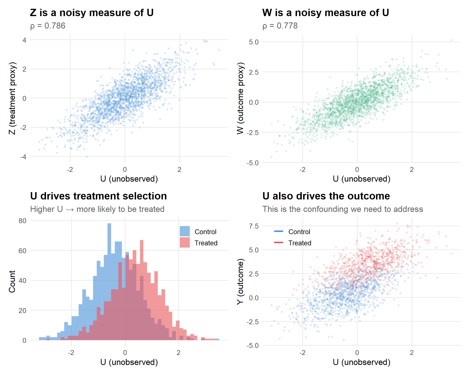
I’m going to simulate data with an unobserved confounder \(U\), a binary treatment \(A\) that depends on \(U\) and \(X\), an outcome \(Y\) that depends on \(A\), \(U\), and \(X\), and two proxies: \(Z\) (treatment-inducing) and \(W\) (outcome-inducing), both noisy measurements of \(U\). Crucially: \(A\) does not cause \(W\) or \(Z\)—they are pre-treatment measurements of the latent confounder, which makes the proxy restrictions hold by construction in this toy world.
Code
simulate_pci_data <-function(n,tau =2,proxy_noise =0.8,seed =NULL) {if (!is.null(seed)) set.seed(seed) X1 <-rnorm(n) X2 <-rbinom(n, 1, 0.4) U <-rnorm(n) Z <- U +rnorm(n, sd = proxy_noise) W <- U +rnorm(n, sd = proxy_noise) lin_A <--0.2+0.9* U +0.5* X1 -0.3* X2 +rnorm(n, sd =0.5) pA <-plogis(lin_A) A <-rbinom(n, 1, pA) Y <-1+ tau * A +1.0* U +0.6* X1 -0.4* X2 +rnorm(n, sd =1)tibble(Y, A, X1, X2, Z, W, U)}
Estimators
Code
estimate_naive <-function(dat) { fit <-lm(Y ~ A + X1 + X2, data = dat)coef(fit)[["A"]]}estimate_oracle <-function(dat) { fit <-lm(Y ~ A + X1 + X2 + U, data = dat)coef(fit)[["A"]]}estimate_proximal_2sls <-function(dat) { stg1 <-lm(W ~ A + Z + X1 + X2, data = dat) dat$W_hat <-predict(stg1) stg2 <-lm(Y ~ A + W_hat + X1 + X2, data = dat)coef(stg2)[["A"]]}boot_estimate <-function(dat, estimator, B =500, seed =1) {set.seed(seed) n <-nrow(dat) draws <-replicate(B, { idx <-sample.int(n, size = n, replace =TRUE)estimator(dat[idx, , drop =FALSE]) })tibble(estimate =mean(draws),se_boot =sd(draws),ci_low =unname(quantile(draws, 0.025)),ci_high =unname(quantile(draws, 0.975)) )}
One simulated dataset (sanity check)
Code
dat1 <-simulate_pci_data(n =2000, tau =2, seed =123)
Before running any estimator, let’s visualize the proxy structure. Hover over points to explore individual observations:
Code
p_uz <-ggplot(dat1, aes(x = U, y = Z, text =paste0("U: ", round(U,2), "<br>Z: ", round(Z,2)))) +geom_point(alpha =0.15, size =0.8, color = pal[1]) +geom_smooth(method ="lm", color = pal[1], se =FALSE) +labs(title ="Z is a noisy measure of U",subtitle =paste0("ρ = ", round(cor(dat1$U, dat1$Z), 3)),x ="U (unobserved)", y ="Z (treatment proxy)")p_uw <-ggplot(dat1, aes(x = U, y = W, text =paste0("U: ", round(U,2), "<br>W: ", round(W,2)))) +geom_point(alpha =0.15, size =0.8, color = pal[3]) +geom_smooth(method ="lm", color = pal[3], se =FALSE) +labs(title ="W is a noisy measure of U",subtitle =paste0("ρ = ", round(cor(dat1$U, dat1$W), 3)),x ="U (unobserved)", y ="W (outcome proxy)")p_ua <-ggplot(dat1, aes(x = U, fill =factor(A))) +geom_histogram(alpha =0.6, position ="identity", bins =50) +scale_fill_manual(values = pal[1:2], labels =c("Control", "Treated"), name =NULL) +labs(title ="U drives treatment selection",subtitle ="Higher U → more likely to be treated",x ="U (unobserved)", y ="Count") +theme(legend.position =c(0.85, 0.85))p_uy <-ggplot(dat1, aes(x = U, y = Y, color =factor(A),text =paste0("U: ", round(U,2), "<br>Y: ", round(Y,2),"<br>A: ", A))) +geom_point(alpha =0.15, size =0.8) +geom_smooth(method ="lm", se =FALSE) +scale_color_manual(values = pal[1:2], labels =c("Control", "Treated"), name =NULL) +labs(title ="U also drives the outcome",subtitle ="This is the confounding we need to address",x ="U (unobserved)", y ="Y (outcome)") +theme(legend.position =c(0.15, 0.85))(p_uz + p_uw) / (p_ua + p_uy)
Figure 2: The proxy structure: Z and W are noisy measurements of U. Hover to inspect individual observations.
The top row shows that \(Z\) and \(W\) are both noisy but informative measurements of \(U\)—exactly the structure PCI needs. The bottom row shows why we need PCI in the first place: \(U\) drives both treatment selection and outcomes, creating confounding that naive regression can’t fix.
The naive regression is biased upward (red) because \(U\) is omitted and positively associated with both \(A\) and \(Y\). The oracle and proximal estimates are close to the truth (green).
Monte Carlo: distribution of estimates
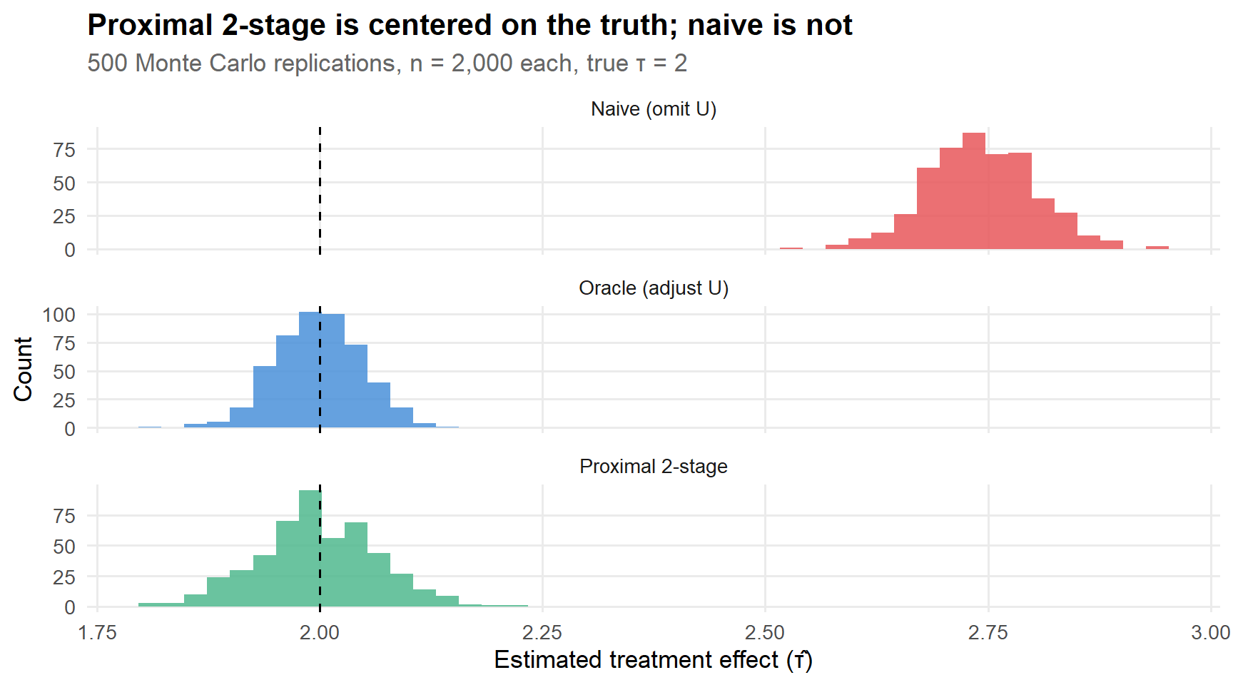
A single dataset is a single draw. Let’s see what happens across 500 replications:
ggplot(mc, aes(x = tau_hat, fill = method)) +geom_histogram(bins =45, alpha =0.85, show.legend =FALSE) +geom_vline(xintercept = tau_true, linetype ="dashed", linewidth =0.6) +facet_wrap(~ method, ncol =1, scales ="free_y") +scale_fill_manual(values = pal[c(2, 1, 3)]) +labs(x ="Estimated treatment effect (τ̂)",y ="Count",title ="Proximal 2-stage is centered on the truth; naive is not",subtitle ="500 Monte Carlo replications, n = 2,000 each, true τ = 2" )
Figure 3: Monte Carlo distributions of treatment effect estimates across 500 replications. The dashed line marks the true τ = 2.
The story is clear: the naive estimator is systematically biased (its distribution is centered above 2), while both the oracle and the proximal estimator are centered on the truth. The proximal estimator is noisier than the oracle—you pay a variance price for not observing \(U\) directly—but it’s unbiased, which is the important thing.
Code
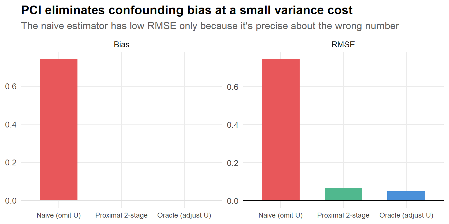
mc_summary |>pivot_longer(cols =c(bias, rmse), names_to ="metric", values_to ="value") |>mutate(metric =recode(metric, bias ="Bias", rmse ="RMSE"),method =factor(method, levels =c("Naive (omit U)", "Proximal 2-stage", "Oracle (adjust U)")) ) |>ggplot(aes(x = method, y = value, fill = method)) +geom_col(width =0.6, show.legend =FALSE) +geom_hline(yintercept =0, linewidth =0.3) +facet_wrap(~ metric, scales ="free_y") +scale_fill_manual(values = pal[c(2, 3, 1)]) +labs(x =NULL, y =NULL,title ="PCI eliminates confounding bias at a small variance cost",subtitle ="The naive estimator has low RMSE only because it's precise about the wrong number") +theme(axis.text.x =element_text(size =9))
Figure 4: Bias and RMSE comparison across estimators.
That last subtitle is the key insight: low RMSE isn’t a virtue if you’re precisely estimating the wrong thing. The naive estimator is biased, and no amount of additional data will fix that.
Bootstrap SEs on one draw
Two-stage procedures with generated regressors can make analytic standard errors subtle. A nonparametric bootstrap is a pragmatic default:
Code
boot_estimate(dat1, estimate_proximal_2sls, B =500, seed =99)
Interactive explorer: what happens when proxies get weaker?
One of the most important practical questions is: how much does the quality of your proxies matter? The answer is “a lot.” Below I’ve pre-computed results across a range of proxy noise levels—use the interactive plot to explore the bias-variance tradeoff.
p_interactive <- proxy_strength_results |>pivot_longer(cols =c(bias, sd, rmse), names_to ="metric", values_to ="value") |>mutate(metric =recode(metric,bias ="Bias",sd ="Std. Dev.",rmse ="RMSE")) |>ggplot(aes(x = proxy_noise, y = value, color = metric,text =paste0("Noise SD: ", proxy_noise,"<br>Corr(U, proxy): ", proxy_corr,"<br>", metric, ": ", round(value, 3)))) +geom_line(linewidth =1) +geom_point(size =2) +geom_hline(yintercept =0, linetype ="dashed", alpha =0.4) +scale_color_manual(values = pal[c(1, 2, 4)], name =NULL) +labs(x ="Proxy noise (SD of measurement error)",y ="Value",title ="Bias stays flat; variance explodes with weak proxies",subtitle ="This is the proximal analogue of the 'weak instruments' problem" ) +theme(legend.position ="top")ggplotly(p_interactive, tooltip ="text") |>layout(hoverlabel =list(bgcolor ="white"))
Figure 5: Effect of proxy noise on the proximal estimator. Hover to see exact values at each noise level.
This is worth internalizing. The proximal estimator stays approximately unbiased even as proxy noise increases (the bridge function is still doing its job), but the variance grows rapidly. At very high noise levels, you’re technically unbiased but your confidence intervals are so wide that the estimate is useless.
Rule of thumb
If the correlation between your proxy \(Z\) and the outcome proxy \(W\) (conditional on \(A\) and \(X\)) is weak, treat the proximal estimates with the same suspicion you’d give a weak-instrument 2SLS estimate. Check the first-stage F-statistic, look at the bootstrap distribution, and don’t over-interpret point estimates with enormous confidence intervals.
Interactive explorer: how does sample size help?
The variance problem above gets better with more data. But how much data do you need? Let’s explore this across different sample sizes and proxy quality levels:
p_nn <- n_noise_results |>ggplot(aes(x = n, y = rmse, color = noise_label,text =paste0("n = ", scales::comma(n),"<br>Proxy noise: ", proxy_noise,"<br>RMSE: ", round(rmse, 3),"<br>Bias: ", round(bias, 3)))) +geom_line(linewidth =1) +geom_point(size =2.5) +scale_x_log10(labels = scales::comma_format()) +scale_color_manual(values = pal, name =NULL) +labs(x ="Sample size (log scale)",y ="RMSE",title ="Better proxies vs. more data: proxy quality wins",subtitle ="Each line is a different proxy noise level; RMSE drops with n but faster with better proxies" ) +theme(legend.position ="top")ggplotly(p_nn, tooltip ="text") |>layout(hoverlabel =list(bgcolor ="white"))
Figure 6: RMSE by sample size and proxy quality. Hover over lines to compare. Better proxies help more than bigger samples.
The takeaway: with strong proxies (low noise), even moderate sample sizes give you good estimates. With weak proxies (high noise), you need a lot of data to compensate—and sometimes the variance is so large that the estimate remains practically useless regardless of \(n\). Investing in better proxies is almost always more productive than collecting more observations.
Part 2: Real-data illustration (wage returns, noisy ability proxies)
For a real dataset, I’ll use wage2 from the wooldridge package (Shea and Brown 2025). This dataset traces back to work on wage equations and unobserved ability, with a classic reference being Blackburn & Neumark (1992) (Blackburn and Neumark 1992).
What I’m doing (and what I’m not claiming)
I’ll illustrate PCI mapping onto a standard economics story:
Treatment\(A\): being a college graduate (constructed from years of schooling \(\geq 16\)).
\(W\): IQ score (IQ) as an outcome-inducing proxy.
\(Z\): knowledge of world-of-work score (KWW) as a treatment-inducing proxy.
Caveat: This is an illustration of the mechanics, not a definitive estimate of the causal return to college. In real labor data, test scores can be affected by education, and both proxies may have direct channels to wages that violate the strict proxy restrictions. Treat this as a worked example, not a policy recommendation.
Standard OLS controlling for demographics but ignoring ability entirely. This is the “hope there’s no omitted variable bias” approach.
Code
ols <-lm(lwage ~ college + exper + tenure + age + married + black + south + urban + sibs + brthord + meduc + feduc,data = w)coeftest(ols, vcov =vcovHC(ols, type ="HC2"))["college", ]
    Estimate   Std. Error      t value     Pr(>|t|)
1.700895e-01 3.544713e-02 4.798401e+00 1.985635e-06
Just adding IQ and KWW as standard controls. This is not proximal inference—it’s what many applied papers do (“control for test scores and hope for the best”).
Code
ols_proxy <-lm(lwage ~ college + IQ + KWW + exper + tenure + age + married + black + south + urban + sibs + brthord + meduc + feduc,data = w)coeftest(ols_proxy, vcov =vcovHC(ols_proxy, type ="HC2"))["college", ]
   Estimate  Std. Error     t value    Pr(>|t|)
0.106224976 0.037555823 2.828455571 0.004821902
The coefficient on college drops when you add IQ and KWW—these proxies are soaking up some omitted-variable bias. But are they soaking up enough?
The PCI approach: use the proxies structurally rather than as direct controls.
Stage 1:\(W = \text{IQ} \sim A + Z + X\), where \(Z = \text{KWW}\).
Stage 2:\(Y = \text{lwage} \sim A + \widehat{\text{IQ}} + X\).
Code
stg1 <-lm(IQ ~ college + KWW + exper + tenure + age + married + black + south + urban + sibs + brthord + meduc + feduc,data = w)w$IQ_hat <-predict(stg1)stg2 <-lm(lwage ~ college + IQ_hat + exper + tenure + age + married + black + south + urban + sibs + brthord + meduc + feduc,data = w)coeftest(stg2, vcov =vcovHC(stg2, type ="HC2"))["college", ]
  Estimate Std. Error    t value   Pr(>|t|)
0.03302397 0.06485348 0.50920886 0.61077891
Proxy strength diagnostic
In this linear setup, we need \(Z\) to have predictive power for \(W\) in Stage 1. Weak relationships → unstable estimates.
Code
summary(stg1)$coefficients["KWW", ]
    Estimate   Std. Error      t value     Pr(>|t|)
5.724527e-01 7.458186e-02 7.675495e+00 6.072347e-14
The partial F-test for adding KWW to the first stage:
Figure 9: Estimated college wage premium under different approaches. Hover for details.
The typical pattern: unadjusted OLS is the largest (ability bias pushes it up), controlling for proxies directly brings it down somewhat, and the proximal 2-stage estimate may adjust further—with a wider confidence interval reflecting the honest uncertainty.
(Set eval: false because I don’t want this post to fail if PCL isn’t installed.)
How I would write this up in a paper
If I were using PCI in an applied project, the write-up would need to be explicit about several things—and reviewers will absolutely ask about each of them:
What latent confounding mechanism \(U\) you are targeting (e.g., “ability,” “severity,” “seller quality”). Vague appeals to “unobserved heterogeneity” aren’t enough; you need a substantive story.
Why the chosen proxies plausibly satisfy the proxy restrictions:
Why is \(W\) not affected by \(A\)? (Timing arguments are strongest here: if \(W\) was measured before treatment, it can’t be affected by treatment.)
Why does \(Z\) not have a direct channel to \(Y\) that bypasses \(A\) and \(U\)?
Ringlein et al. (2025) offer a helpful discussion of proxy selection strategies, including the use of temporal ordering as a guide.
Proxy strength / information content. Completeness is not testable, but weak proxy relationships are a red flag. Report the first-stage F-statistic or partial \(R^2\) of \(Z\) on \(W\).
Modeling choices for the bridge function:
Linear vs. nonlinear (do you believe a linear bridge is adequate?).
Whether to include interactions (\(A \times W\), which allows heterogeneous effects).
Sensitivity to specification.
Comparison with alternative strategies: show results from naive OLS, direct proxy adjustment, and (if applicable) IV or difference-in-differences. Triangulation builds credibility.
PCI trades one untestable assumption (no unmeasured confounding) for different untestable assumptions (proxy restrictions + completeness). Whether that trade is worth it depends on domain knowledge and the credibility of your proxy story. If you can’t articulate why your proxies satisfy the required exclusion restrictions, PCI won’t save you.
You need to argue why a variable belongs in \(Z\) (treatment-inducing) versus \(W\) (outcome-inducing). Getting this wrong can silently invalidate the estimand (Tchetgen Tchetgen et al. 2024). In some settings the classification is natural (a pre-treatment test score vs. a post-treatment biomarker), but in others it requires real thought. If you’re unsure, try both assignments and see if the results are qualitatively similar—large sensitivity to proxy role assignment is a red flag.
Even in the parametric linear case, if \(Z\) barely predicts \(W\) (conditional on \(A\) and \(X\)), the second stage can be wildly unstable. We saw this in the simulation. Check your first-stage diagnostics seriously.
The linear two-stage approach is clean and easy, but it assumes the bridge function is linear. For binary outcomes, count data, or survival times, you need different machinery. Liu et al. (2025) develop regression-based proximal methods for GLMs, and there’s growing work on survival outcomes and censored data.
If you need nonparametric flexibility, there are kernel-based and neural-network approaches for estimating the bridge function (Cui et al. 2024; Ringlein et al. 2025). But the bridge equation is an inverse problem, and inverse problems are inherently unstable without regularization. Plan for careful tuning and honest uncertainty quantification.
If you have more than one proxy of each type, use them. Additional proxies strengthen the completeness condition and can improve precision. In the linear case, just add more variables to the first stage.
A subtle but important point, emphasized by Ringlein et al. (2025): PCI requires a specific conceptualization of what \(U\) is and why your proxies are informative about that specific confounder. It does not protect against confounders you haven’t thought of. This is a feature, not a bug—it forces you to be explicit—but it means PCI is not a general-purpose cure for all unmeasured confounding.
Where the field is heading
PCI is a fast-moving area. A few directions I’m watching:
Doubly robust proximal estimators that combine bridge function estimation with inverse weighting, providing robustness to partial model misspecification.
Extensions to time-varying treatments and longitudinal settings, building on the g-computation tradition.
Sensitivity analysis and partial identification for settings where proxy assumptions are approximately but not exactly satisfied. Ringlein et al. (2025) highlight recent work on “fortified” proximal estimators that remain informative even with some proxy violations.
Connections to measurement error and data fusion, where the proxy structure naturally arises from linking imperfect data sources.
Software development: the PCL package is a start, and the pci2s package extends proximal methods to survival data. I expect more mature tooling in the next year or two.
The bottom line
Proximal causal inference is one of the more elegant ideas to emerge from the causal inference literature in recent years. It gives you a principled way to handle a specific and common type of unmeasured confounding—the kind where you can’t measure the confounder directly, but you can find proxy variables that are “noisy shadows” of it.
The catch is that PCI’s assumptions are different from, not weaker than, the standard selection-on-observables assumptions. You trade “I’ve measured all confounders” for “I’ve found two proxies that satisfy specific exclusion restrictions with respect to an unobserved confounder I’ve explicitly conceptualized.” Whether that’s a good trade depends entirely on your setting and your domain knowledge.
When the proxy story is credible, PCI can give you identification where no other observational method can. When it’s not, it gives you a precisely wrong answer with a veneer of sophistication. Use it wisely.
Blackburn, McKinley, and David Neumark. 1992. “Unobserved Ability, Efficiency Wages, and Interindustry Wage Differentials.”The Quarterly Journal of Economics 107 (4): 1421–36. https://doi.org/10.2307/2118394.
Cui, Yifan, Hongming Pu, Xu Shi, Wang Miao, and Eric J. Tchetgen Tchetgen. 2024. “Semiparametric Proximal Causal Inference.”Journal of the American Statistical Association 119 (546): 1348–59. https://doi.org/10.1080/01621459.2023.2191817.
Liu, Jiewen, Chan Park, Kendrick Li, and Eric J. Tchetgen Tchetgen. 2025. “Regression-Based Proximal Causal Inference.”American Journal of Epidemiology 194 (7): 2030–36. https://doi.org/10.1093/aje/kwae370.
Miao, Wang, Zhi Geng, and Eric J. Tchetgen Tchetgen. 2018. “Identifying Causal Effects with Proxy Variables of an Unmeasured Confounder.”Biometrika 105 (4): 987–93. https://doi.org/10.1093/biomet/asy038.
Ringlein, Grace V, Trang Quynh Nguyen, Peter P Zandi, Elizabeth A Stuart, and Harsh Parikh. 2025. “Demystifying Proximal Causal Inference.”arXiv Preprint arXiv:2512.24413.
Shea, Justin M., and Kennth H. Brown. 2025. Wooldridge: 115 Data Sets from “Introductory Econometrics: A Modern Approach, 7e” by Jeffrey m. Wooldridge. https://cran.r-project.org/package=wooldridge.
Tchetgen Tchetgen, Eric J., Andrew Ying, Yifan Cui, Xu Shi, and Wang Miao. 2024. “An Introduction to Proximal Causal Inference.”Statistical Science 39 (3): 375–90. https://doi.org/10.1214/23-STS911.
Zivich, Paul N., Stephen R. Cole, Jessie K. Edwards, Grace E. Mulholland, Bonnie E. Shook-Sa, and Eric J. Tchetgen Tchetgen. 2023. “Introducing Proximal Causal Inference for Epidemiologists.”American Journal of Epidemiology 192 (7): 1224–27. https://doi.org/10.1093/aje/kwad077.
Source Code
---title: "Proximal Causal Inference: A Practical Guide (with R Code)"date: 2025-11-18author: "Felicia Nguyen"description: "How to estimate causal effects with unmeasured confounding using proxy variables, with a worked simulation and a real-data walkthrough in R."categories: [Causal Inference, Econometrics, Statistics, R]format: html: toc: true toc-depth: 3 code-fold: show code-tools: trueexecute: echo: true warning: false message: falsebibliography: references.bib---## Why I care about proximal causal inferenceMost of the causal estimators I reach for day-to-day---regression adjustment, matching, inverse probability weighting, doubly robust estimators---lean heavily on a version of *conditional exchangeability* (a.k.a. "selection on observables" or "no unmeasured confounding"):$$Y(a) \perp\!\!\!\perp A \mid X$$where $A$ is the treatment, $Y$ is the outcome, $X$ are measured covariates, and $Y(a)$ is the potential outcome under treatment level $a$.The problem is that in a lot of the observational work I care about, I don't fully buy $Y(a) \perp\!\!\!\perp A \mid X$. Sometimes the missing piece is a substantively important confounder $U$ that is hard (or impossible) to measure well: ability, motivation, latent health status, risk preference, clinician judgment, seller quality, algorithmic recommendation intensity, etc. We've all been in that seminar where someone raises their hand and says "but what about unobserved heterogeneity?"---and the presenter takes a long sip of water.**Proximal causal inference** (PCI) is one of the cleanest frameworks I know for making progress in exactly that setting: *unmeasured confounding exists*, but we have **proxy variables** that carry information about the unmeasured confounder(s). The canonical identification results trace back to proxy-variable work in Biometrika and were later organized into a "proximal g-formula" framework [@miao2018proxy; @tchetgen2024intro]. The basic idea has been around for a while, but there's been an explosion of methodological work in the last few years, including extensions to survival data, mediation, time-varying treatments, and semiparametric estimation [@cui2024semiparametric; @liu2025regression_pci; @ringlein2025demystifying].This post is my attempt to give a working, applied introduction:1. The setup and the assumptions (in plain language).2. The "bridge function" trick that makes identification work.3. A full implementation in **R**: - a simulation where we *know* the truth, - a real-data illustration using the `wage2` dataset.4. Practical tips, diagnostics, and failure modes.I'll keep the discussion at the "what I need to run this responsibly" level, and I'll flag where things can go off the rails. PCI is powerful, but it is emphatically not a free lunch---it trades one set of untestable assumptions for another, and whether that trade is worth it depends entirely on your domain knowledge.::: {.callout-tip}## The one-sentence pitchIf you have a confounder you can't measure but you *can* find two proxy variables that are "noisy shadows" of it, proximal causal inference lets you recover the causal effect---under assumptions that are different from (not weaker than) the standard "no unmeasured confounding" assumption.:::---## The proximal setup in one picturePCI sits in the following data structure:- $A$: treatment / exposure- $Y$: outcome- $X$: measured covariates we're comfortable adjusting for- $U$: *unmeasured* confounder (latent)- $Z$: a **treatment-inducing proxy** (a.k.a. treatment confounding proxy, or negative control exposure)- $W$: an **outcome-inducing proxy** (a.k.a. outcome confounding proxy, or negative control outcome)A simple DAG is:```{mermaid}%%| label: fig-dag%%| fig-cap: "Proximal causal inference DAG. Solid arrows represent allowed (and present) causal relationships. The key exclusion restrictions are the *absent* arrows: no Z → Y and no W → A."%%| fig-width: 7graph TD Z["<b>Z</b><br/><i>treatment proxy</i>"] W["<b>W</b><br/><i>outcome proxy</i>"] U(("<b>U</b><br/><i>unobserved</i>")) A["<b>A</b><br/><i>treatment</i>"] Y((("<b>Y</b><br/><i>outcome</i>"))) X["<b>X</b><br/><i>covariates</i>"] U --> Z U --> W U --> A U --> Y U <--> X Z -.-> A W -.-> Y A --> Y X --> A X --> Y style U fill:#F5A623,stroke:#D4891A,color:#fff,stroke-width:2px style A fill:#4A90D9,stroke:#3570A8,color:#fff,stroke-width:2px style Y fill:#4A90D9,stroke:#3570A8,color:#fff,stroke-width:2px style Z fill:#50B88E,stroke:#3D9A73,color:#fff,stroke-width:2px style W fill:#50B88E,stroke:#3D9A73,color:#fff,stroke-width:2px style X fill:#999,stroke:#777,color:#fff,stroke-width:1px```The double circle around $U$ is the visual convention for "unobserved." Notice the arrows that are *present* and the ones that are *absent*---the absent arrows are doing all the identification work:- **$Z \to A$ exists but $Z \to Y$ does not.** The treatment proxy *may or may not* cause treatment (that's fine), but it has no direct effect on the outcome once you condition on $A$, $U$, and $X$. This is the treatment-proxy exclusion restriction: $Y \perp\!\!\!\perp Z \mid A, U, X$.- **$W \to Y$ exists but $W \to A$ does not.** The outcome proxy *may or may not* affect the outcome (that's fine), but it doesn't independently drive treatment assignment once you condition on $U$ and $X$. This is the outcome-proxy exclusion restriction: $W \perp\!\!\!\perp A \mid U, X$.If this looks vaguely familiar, it should. The idea is conceptually related to instrumental variables (IV), but the mechanics are different. In IV, you need an instrument that affects treatment but not the outcome (except through treatment). In PCI, you need *two* proxies that each satisfy different exclusion restrictions relative to the unobserved confounder. The identification argument goes through a "bridge function" rather than through an exclusion restriction on the outcome equation.::: {.callout-note}## Terminology noteThe naming conventions in this literature are... not ideal. Different papers call these proxies different things: "treatment-inducing" vs. "outcome-inducing" [@tchetgen2024intro], "type Z" vs. "type W" [@miao2018proxy], or "negative control exposure" vs. "negative control outcome" [@zivich2023pci_epi]. @ringlein2025demystifying note that the names reference the *unrestricted* relationships (Z may cause A; W may cause Y), which is arguably backwards from how you'd want to think about them. I'll use the $Z$/$W$ notation throughout and try to be explicit about which restriction applies to which proxy.:::---## Assumptions: what replaces exchangeability?I'll state the assumptions in the way I find easiest to reason about. Notation varies across papers, but the core content is consistent [@tchetgen2024intro; @miao2018proxy; @ringlein2025demystifying].::: {.panel-tabset}### Consistency & positivityThese are the same assumptions you need for any causal estimand---nothing proximal-specific here.- **Consistency:** $Y = Y(A)$. The observed outcome equals the potential outcome under the observed treatment.- **Positivity:** treatment variation exists at the relevant covariate / confounder levels.### Proxy exclusion restrictionsThese are the key proximal ingredients, and they're where all the identification power (and all the assumptions) live.**Outcome-proxy restriction (for $W$):** $W$ is not affected by $A$, and conditional on $U$ and $X$, it is independent of treatment assignment:$$W \perp\!\!\!\perp A \mid U, X$$In words: once you knew the latent confounder $U$ (and $X$), $W$ would be irrelevant for predicting $A$. Think of $W$ as a "downstream consequence" of $U$ that doesn't go through $A$.**Treatment-proxy restriction (for $Z$):** $Z$ is "as-good-as-irrelevant" for the outcome once we know the treatment and the confounder:$$Y \perp\!\!\!\perp Z \mid A, U, X$$In words: $Z$ doesn't have a direct causal path to $Y$ that isn't already captured by $A$, $U$, and $X$. Think of $Z$ as something that predicts treatment *because* it's related to $U$, but that has no independent effect on the outcome.These are conceptually similar to negative control restrictions, which is why PCI is often taught as a "beyond detection" use of negative controls [@zivich2023pci_epi; @tchetgen2024intro].### Completeness / rankPCI also needs a kind of "no degeneracy" condition ensuring that the proxies carry enough information about $U$ to identify the bridge function. In econometrics terms, it's close in spirit to the completeness conditions that show up in nonparametric IV (NPIV): the conditional distribution of $W$ (or $Z$) given $(A, X, Z)$ must be "rich enough" that a certain integral equation has a unique solution.This is one of the reasons proximal estimation can be **ill-posed** and can benefit from regularization in flexible settings [@tchetgen2024intro; @cui2024semiparametric]. In the linear case, it reduces to a familiar rank condition (essentially: $Z$ must have predictive power for $W$ conditional on $A$ and $X$, which is analogous to "instrument relevance" in IV).I won't re-derive completeness here, but I *will* take it seriously in the implementation section: weak proxy relationships tend to blow up estimates, just like weak instruments blow up 2SLS.### How it compares to IV|| **Instrumental Variables** | **Proximal Causal Inference** ||---|---|---|| **What you need** | 1 instrument $Z$ | 2 proxies: $Z$ (treatment) + $W$ (outcome) || **Key restriction** | $Z \to Y$ only through $A$ | $Z \not\to Y$ given $A, U, X$; $W \not\to A$ given $U, X$ || **What's latent** | Nothing (confounders assumed measured) | $U$ is explicitly unobserved || **First stage predicts** | Treatment $A$ | Outcome proxy $W$ || **Estimand** | LATE (with heterogeneity) | ATE (under bridge function) || **Weak instrument analogue** | Weak $Z \to A$ | Weak $Z \to W \mid A, X$ |:::---## Identification: the bridge function trickThe core move in PCI is to introduce an **outcome confounding bridge function** $h(\cdot)$ that "translates" the outcome $Y$ into something that can be written as a function of the observed proxy $W$.The defining equation is:$$\mathbb{E}\left[Y \mid A=a, Z=z, X=x\right]=\mathbb{E}\left[h(W, a, x) \mid A=a, Z=z, X=x\right]$$If such an $h$ exists (and the completeness conditions hold), then the causal estimand becomes:$$\mathbb{E}[Y(a)] = \mathbb{E}\left[h(W, a, X)\right]$$and the ATE is $\mathbb{E}[h(W,1,X) - h(W,0,X)]$.This is the "proximal g-formula" [@tchetgen2024intro; @miao2018proxy].The intuition: $h$ is a function that, when evaluated at the observed proxy $W$ (instead of the unobserved $U$), gives you the right answer *on average*. The bridge function "bridges" the gap between what you can observe ($W$) and what you need ($U$). It's solving an inverse problem: recovering a function of a latent variable from its noisy proxies.For an applied workflow, the main question becomes: **how do I parameterize or estimate $h$ in a way that is stable enough to use?** That's where the two-stage regressions come in.---## Estimation: proximal two-stage least squaresTo keep things concrete, suppose $A$ is binary, $Y$ is continuous, and $W$ and $Z$ are continuous proxies. A convenient (and common) working model is a linear bridge:$$h(W, A, X) = \beta_0 + \beta_A A + \beta_W W + \beta_X^\top X$$Plugging this into the bridge equation implies:$$\mathbb{E}[Y \mid A, Z, X]=\beta_0 + \beta_A A + \beta_W \mathbb{E}[W \mid A, Z, X] + \beta_X^\top X$$This suggests a **two-stage regression**:1. **Stage 1:** Regress $W$ on $(A, Z, X)$ to get $\widehat{W} = \widehat{\mathbb{E}}[W \mid A, Z, X]$.2. **Stage 2:** Regress $Y$ on $(A, \widehat{W}, X)$.Under the linear bridge specification, the ATE is simply $\beta_A$, because $h(W,1,X) - h(W,0,X) = \beta_A$.This "proximal 2SLS" flavor is implemented in the `PCL` package [@PCLpkg] and appears as a special case in the broader proximal literature [@tchetgen2024intro; @liu2025regression_pci].::: {.callout-warning}## This is NOT standard IVI want to be very explicit about this, because it trips people up. We are **not** using $Z$ as an instrument for $A$. We are using $Z$ to help recover the confounder information that is latent in $W$, so that $h(W, A, X)$ can be learned. The first stage predicts $W$ (the outcome proxy), not $A$ (the treatment). The exclusion restrictions are different from IV. The estimand is different from IV. If you're coming from an econometrics background where 2SLS = IV, you need to reset your priors here.:::---## R setup```{r}#| label: setuplibrary(dplyr)library(tidyr)library(ggplot2)library(purrr)library(broom)library(lmtest)library(sandwich)library(patchwork)library(plotly)library(reactable)library(wooldridge)theme_set(theme_minimal(base_size =13) +theme(plot.title =element_text(face ="bold"),plot.subtitle =element_text(color ="grey40"),panel.grid.minor =element_blank() ))pal <-c("#4A90D9", "#E8575A", "#50B88E", "#F5A623")```---## Part 1: Simulation---where we know the truth### Data-generating processI'm going to simulate data with an unobserved confounder $U$, a binary treatment $A$ that depends on $U$ and $X$, an outcome $Y$ that depends on $A$, $U$, and $X$, and two proxies: $Z$ (treatment-inducing) and $W$ (outcome-inducing), both noisy measurements of $U$. Crucially: $A$ does not cause $W$ or $Z$---they are pre-treatment measurements of the latent confounder, which makes the proxy restrictions hold by construction in this toy world.```{r}#| label: sim-functionssimulate_pci_data <-function(n,tau =2,proxy_noise =0.8,seed =NULL) {if (!is.null(seed)) set.seed(seed) X1 <-rnorm(n) X2 <-rbinom(n, 1, 0.4) U <-rnorm(n) Z <- U +rnorm(n, sd = proxy_noise) W <- U +rnorm(n, sd = proxy_noise) lin_A <--0.2+0.9* U +0.5* X1 -0.3* X2 +rnorm(n, sd =0.5) pA <-plogis(lin_A) A <-rbinom(n, 1, pA) Y <-1+ tau * A +1.0* U +0.6* X1 -0.4* X2 +rnorm(n, sd =1)tibble(Y, A, X1, X2, Z, W, U)}```### Estimators```{r}#| label: estimatorsestimate_naive <-function(dat) { fit <-lm(Y ~ A + X1 + X2, data = dat)coef(fit)[["A"]]}estimate_oracle <-function(dat) { fit <-lm(Y ~ A + X1 + X2 + U, data = dat)coef(fit)[["A"]]}estimate_proximal_2sls <-function(dat) { stg1 <-lm(W ~ A + Z + X1 + X2, data = dat) dat$W_hat <-predict(stg1) stg2 <-lm(Y ~ A + W_hat + X1 + X2, data = dat)coef(stg2)[["A"]]}boot_estimate <-function(dat, estimator, B =500, seed =1) {set.seed(seed) n <-nrow(dat) draws <-replicate(B, { idx <-sample.int(n, size = n, replace =TRUE)estimator(dat[idx, , drop =FALSE]) })tibble(estimate =mean(draws),se_boot =sd(draws),ci_low =unname(quantile(draws, 0.025)),ci_high =unname(quantile(draws, 0.975)) )}```### One simulated dataset (sanity check)```{r}#| label: sim-onedat1 <-simulate_pci_data(n =2000, tau =2, seed =123)```Before running any estimator, let's visualize the proxy structure. Hover over points to explore individual observations:```{r}#| label: fig-proxy-structure#| fig-cap: "The proxy structure: Z and W are noisy measurements of U. Hover to inspect individual observations."#| fig-width: 10#| fig-height: 8p_uz <-ggplot(dat1, aes(x = U, y = Z, text =paste0("U: ", round(U,2), "<br>Z: ", round(Z,2)))) +geom_point(alpha =0.15, size =0.8, color = pal[1]) +geom_smooth(method ="lm", color = pal[1], se =FALSE) +labs(title ="Z is a noisy measure of U",subtitle =paste0("ρ = ", round(cor(dat1$U, dat1$Z), 3)),x ="U (unobserved)", y ="Z (treatment proxy)")p_uw <-ggplot(dat1, aes(x = U, y = W, text =paste0("U: ", round(U,2), "<br>W: ", round(W,2)))) +geom_point(alpha =0.15, size =0.8, color = pal[3]) +geom_smooth(method ="lm", color = pal[3], se =FALSE) +labs(title ="W is a noisy measure of U",subtitle =paste0("ρ = ", round(cor(dat1$U, dat1$W), 3)),x ="U (unobserved)", y ="W (outcome proxy)")p_ua <-ggplot(dat1, aes(x = U, fill =factor(A))) +geom_histogram(alpha =0.6, position ="identity", bins =50) +scale_fill_manual(values = pal[1:2], labels =c("Control", "Treated"), name =NULL) +labs(title ="U drives treatment selection",subtitle ="Higher U → more likely to be treated",x ="U (unobserved)", y ="Count") +theme(legend.position =c(0.85, 0.85))p_uy <-ggplot(dat1, aes(x = U, y = Y, color =factor(A),text =paste0("U: ", round(U,2), "<br>Y: ", round(Y,2),"<br>A: ", A))) +geom_point(alpha =0.15, size =0.8) +geom_smooth(method ="lm", se =FALSE) +scale_color_manual(values = pal[1:2], labels =c("Control", "Treated"), name =NULL) +labs(title ="U also drives the outcome",subtitle ="This is the confounding we need to address",x ="U (unobserved)", y ="Y (outcome)") +theme(legend.position =c(0.15, 0.85))(p_uz + p_uw) / (p_ua + p_uy)```The top row shows that $Z$ and $W$ are both noisy but informative measurements of $U$---exactly the structure PCI needs. The bottom row shows why we need PCI in the first place: $U$ drives both treatment selection and outcomes, creating confounding that naive regression can't fix.Now let's see what the estimators give us:```{r}#| label: sim-one-resultsone_run <-tibble(Method =c("Naive (no U)", "Oracle (adjust U)", "Proximal 2-stage"),Estimate =c(estimate_naive(dat1),estimate_oracle(dat1),estimate_proximal_2sls(dat1) ),`Bias (τ = 2)`= Estimate -2)reactable( one_run,columns =list(Method =colDef(minWidth =180),Estimate =colDef(format =colFormat(digits =3)),`Bias (τ = 2)`=colDef(format =colFormat(digits =3),style =function(value) { color <-if (abs(value) >0.2) "#E8575A"else"#50B88E"list(color = color, fontWeight ="bold") } ) ),striped =TRUE,highlight =TRUE,bordered =TRUE,compact =TRUE)```The naive regression is biased upward (red) because $U$ is omitted and positively associated with both $A$ and $Y$. The oracle and proximal estimates are close to the truth (green).### Monte Carlo: distribution of estimatesA single dataset is a single draw. Let's see what happens across 500 replications:```{r}#| label: sim-mc#| cache: trueset.seed(2026)B <-500n <-2000tau_true <-2mc <-map_dfr(seq_len(B), function(b) { dat <-simulate_pci_data(n = n, tau = tau_true)tibble(b = b,naive =estimate_naive(dat),oracle =estimate_oracle(dat),prox2s =estimate_proximal_2sls(dat) )}) |>pivot_longer(cols =c(naive, oracle, prox2s),names_to ="method",values_to ="tau_hat") |>mutate(method =recode(method,naive ="Naive (omit U)",oracle ="Oracle (adjust U)",prox2s ="Proximal 2-stage"))``````{r}#| label: sim-mc-summarymc_summary <- mc |>group_by(method) |>summarize(mean_est =mean(tau_hat),bias =mean(tau_hat) - tau_true,sd =sd(tau_hat),rmse =sqrt(mean((tau_hat - tau_true)^2)),.groups ="drop" )reactable( mc_summary |>mutate(across(where(is.numeric), \(x) round(x, 4))),columns =list(method =colDef(name ="Method", minWidth =170),mean_est =colDef(name ="Mean τ̂"),bias =colDef(name ="Bias",style =function(value) { color <-if (abs(value) >0.1) "#E8575A"else"#50B88E"list(color = color, fontWeight ="bold") }),sd =colDef(name ="SD"),rmse =colDef(name ="RMSE") ),striped =TRUE, highlight =TRUE, bordered =TRUE, compact =TRUE)``````{r}#| label: fig-mc-distributions#| fig-cap: "Monte Carlo distributions of treatment effect estimates across 500 replications. The dashed line marks the true τ = 2."#| fig-width: 9#| fig-height: 5ggplot(mc, aes(x = tau_hat, fill = method)) +geom_histogram(bins =45, alpha =0.85, show.legend =FALSE) +geom_vline(xintercept = tau_true, linetype ="dashed", linewidth =0.6) +facet_wrap(~ method, ncol =1, scales ="free_y") +scale_fill_manual(values = pal[c(2, 1, 3)]) +labs(x ="Estimated treatment effect (τ̂)",y ="Count",title ="Proximal 2-stage is centered on the truth; naive is not",subtitle ="500 Monte Carlo replications, n = 2,000 each, true τ = 2" )```The story is clear: the naive estimator is systematically biased (its distribution is centered above 2), while both the oracle and the proximal estimator are centered on the truth. The proximal estimator is noisier than the oracle---you pay a variance price for not observing $U$ directly---but it's *unbiased*, which is the important thing.```{r}#| label: fig-mc-bias-variance#| fig-cap: "Bias and RMSE comparison across estimators."#| fig-width: 8#| fig-height: 4mc_summary |>pivot_longer(cols =c(bias, rmse), names_to ="metric", values_to ="value") |>mutate(metric =recode(metric, bias ="Bias", rmse ="RMSE"),method =factor(method, levels =c("Naive (omit U)", "Proximal 2-stage", "Oracle (adjust U)")) ) |>ggplot(aes(x = method, y = value, fill = method)) +geom_col(width =0.6, show.legend =FALSE) +geom_hline(yintercept =0, linewidth =0.3) +facet_wrap(~ metric, scales ="free_y") +scale_fill_manual(values = pal[c(2, 3, 1)]) +labs(x =NULL, y =NULL,title ="PCI eliminates confounding bias at a small variance cost",subtitle ="The naive estimator has low RMSE only because it's precise about the wrong number") +theme(axis.text.x =element_text(size =9))```That last subtitle is the key insight: low RMSE isn't a virtue if you're precisely estimating the wrong thing. The naive estimator is biased, and no amount of additional data will fix that.### Bootstrap SEs on one drawTwo-stage procedures with generated regressors can make analytic standard errors subtle. A nonparametric bootstrap is a pragmatic default:```{r}#| label: sim-bootboot_estimate(dat1, estimate_proximal_2sls, B =500, seed =99)```---### Interactive explorer: what happens when proxies get weaker?One of the most important practical questions is: how much does the quality of your proxies matter? The answer is "a lot." Below I've pre-computed results across a range of proxy noise levels---use the interactive plot to explore the bias-variance tradeoff.```{r}#| label: sim-proxy-strength#| cache: truenoise_levels <-seq(0.2, 3.5, by =0.2)n_sim <-2000B_sim <-300set.seed(42)proxy_strength_results <-map_dfr(noise_levels, function(noise) { ests <-replicate(B_sim, { d <-simulate_pci_data(n = n_sim, tau =2, proxy_noise = noise)estimate_proximal_2sls(d) })tibble(proxy_noise = noise,proxy_corr =round(1/sqrt(1+ noise^2), 3), # theoretical corr(U, proxy)mean_est =mean(ests),bias =mean(ests) - tau_true,sd =sd(ests),rmse =sqrt(mean((ests - tau_true)^2)) )})``````{r}#| label: fig-proxy-strength-interactive#| fig-cap: "Effect of proxy noise on the proximal estimator. Hover to see exact values at each noise level."#| fig-height: 5p_interactive <- proxy_strength_results |>pivot_longer(cols =c(bias, sd, rmse), names_to ="metric", values_to ="value") |>mutate(metric =recode(metric,bias ="Bias",sd ="Std. Dev.",rmse ="RMSE")) |>ggplot(aes(x = proxy_noise, y = value, color = metric,text =paste0("Noise SD: ", proxy_noise,"<br>Corr(U, proxy): ", proxy_corr,"<br>", metric, ": ", round(value, 3)))) +geom_line(linewidth =1) +geom_point(size =2) +geom_hline(yintercept =0, linetype ="dashed", alpha =0.4) +scale_color_manual(values = pal[c(1, 2, 4)], name =NULL) +labs(x ="Proxy noise (SD of measurement error)",y ="Value",title ="Bias stays flat; variance explodes with weak proxies",subtitle ="This is the proximal analogue of the 'weak instruments' problem" ) +theme(legend.position ="top")ggplotly(p_interactive, tooltip ="text") |>layout(hoverlabel =list(bgcolor ="white"))```This is worth internalizing. The proximal estimator stays approximately unbiased even as proxy noise increases (the bridge function is still doing its job), but the *variance* grows rapidly. At very high noise levels, you're technically unbiased but your confidence intervals are so wide that the estimate is useless.::: {.callout-tip}## Rule of thumbIf the correlation between your proxy $Z$ and the outcome proxy $W$ (conditional on $A$ and $X$) is weak, treat the proximal estimates with the same suspicion you'd give a weak-instrument 2SLS estimate. Check the first-stage F-statistic, look at the bootstrap distribution, and don't over-interpret point estimates with enormous confidence intervals.:::### Interactive explorer: how does sample size help?The variance problem above gets better with more data. But *how much* data do you need? Let's explore this across different sample sizes and proxy quality levels:```{r}#| label: sim-n-vs-noise#| cache: truen_levels <-c(500, 1000, 2000, 5000, 10000)noise_grid <-c(0.5, 0.8, 1.5, 2.5)B_grid <-200set.seed(2025)n_noise_results <-expand.grid(n = n_levels, proxy_noise = noise_grid) |>as_tibble() |>mutate(row =row_number()) |>pmap_dfr(function(n, proxy_noise, row) { ests <-replicate(B_grid, { d <-simulate_pci_data(n = n, tau =2, proxy_noise = proxy_noise)estimate_proximal_2sls(d) })tibble(n = n,proxy_noise = proxy_noise,noise_label =paste0("Proxy noise = ", proxy_noise),bias =mean(ests) - tau_true,sd =sd(ests),rmse =sqrt(mean((ests - tau_true)^2)) ) })``````{r}#| label: fig-n-vs-noise#| fig-cap: "RMSE by sample size and proxy quality. Hover over lines to compare. Better proxies help more than bigger samples."#| fig-height: 5p_nn <- n_noise_results |>ggplot(aes(x = n, y = rmse, color = noise_label,text =paste0("n = ", scales::comma(n),"<br>Proxy noise: ", proxy_noise,"<br>RMSE: ", round(rmse, 3),"<br>Bias: ", round(bias, 3)))) +geom_line(linewidth =1) +geom_point(size =2.5) +scale_x_log10(labels = scales::comma_format()) +scale_color_manual(values = pal, name =NULL) +labs(x ="Sample size (log scale)",y ="RMSE",title ="Better proxies vs. more data: proxy quality wins",subtitle ="Each line is a different proxy noise level; RMSE drops with n but faster with better proxies" ) +theme(legend.position ="top")ggplotly(p_nn, tooltip ="text") |>layout(hoverlabel =list(bgcolor ="white"))```The takeaway: with strong proxies (low noise), even moderate sample sizes give you good estimates. With weak proxies (high noise), you need a *lot* of data to compensate---and sometimes the variance is so large that the estimate remains practically useless regardless of $n$. Investing in better proxies is almost always more productive than collecting more observations.---## Part 2: Real-data illustration (wage returns, noisy ability proxies)For a real dataset, I'll use `wage2` from the `wooldridge` package [@wooldridgepkg]. This dataset traces back to work on wage equations and unobserved ability, with a classic reference being Blackburn & Neumark (1992) [@blackburn1992ability].### What I'm doing (and what I'm *not* claiming)I'll illustrate PCI mapping onto a standard economics story:- **Treatment** $A$: being a college graduate (constructed from years of schooling $\geq 16$).- **Outcome** $Y$: log wage (`lwage`).- **Unobserved confounder** $U$: latent "ability" / productivity.- **Proxies:** - $W$: IQ score (`IQ`) as an outcome-inducing proxy. - $Z$: knowledge of world-of-work score (`KWW`) as a treatment-inducing proxy.**Caveat:** This is an *illustration of the mechanics*, not a definitive estimate of the causal return to college. In real labor data, test scores can be affected by education, and both proxies may have direct channels to wages that violate the strict proxy restrictions. Treat this as a worked example, not a policy recommendation.### Load and prepare the data```{r}#| label: wage2-datadata("wage2", package ="wooldridge")w <- wage2 |>transmute( lwage, educ,college =as.integer(educ >=16), IQ, KWW, exper, tenure, age, married, black, south, urban, sibs, brthord, meduc, feduc ) |>na.omit()``````{r}#| label: wage2-summaryw |>summarize(n =n(),college_rate =mean(college),mean_lwage =mean(lwage),sd_lwage =sd(lwage),cor_IQ_KWW =cor(IQ, KWW) )```Let's explore the proxy relationships interactively:```{r}#| label: fig-wage2-proxies-interactive#| fig-cap: "The proxy structure in the wage data. Hover to inspect individual observations."#| fig-height: 5p_wage_iq <-ggplot(w, aes(x = IQ, y = lwage, color =factor(college),text =paste0("IQ: ", IQ, "<br>Log wage: ", round(lwage, 2),"<br>College: ", ifelse(college, "Yes", "No"),"<br>Educ: ", educ, " yrs"))) +geom_point(alpha =0.4, size =1.2) +geom_smooth(method ="lm", se =FALSE) +scale_color_manual(values = pal[1:2], labels =c("No college", "College"), name =NULL) +labs(x ="IQ score (W)", y ="Log wage",title ="IQ predicts wages (and differs by education)") +theme(legend.position ="top")ggplotly(p_wage_iq, tooltip ="text") |>layout(hoverlabel =list(bgcolor ="white"))``````{r}#| label: fig-wage2-kww-iq-interactive#| fig-cap: "KWW and IQ are correlated through latent ability. Hover to inspect."#| fig-height: 4.5p_kww <-ggplot(w, aes(x = KWW, y = IQ,text =paste0("KWW: ", KWW, "<br>IQ: ", IQ,"<br>College: ", ifelse(college, "Yes", "No")))) +geom_point(alpha =0.4, size =1.2, color = pal[3]) +geom_smooth(method ="lm", color = pal[3], se =FALSE) +labs(x ="KWW score (Z)", y ="IQ score (W)",title ="KWW and IQ are correlated",subtitle =paste0("ρ = ", round(cor(w$KWW, w$IQ), 3)))ggplotly(p_kww, tooltip ="text") |>layout(hoverlabel =list(bgcolor ="white"))```---### Estimation: three approaches::: {.panel-tabset}#### OLS (no proxies)Standard OLS controlling for demographics but ignoring ability entirely. This is the "hope there's no omitted variable bias" approach.```{r}#| label: wage2-olsols <-lm(lwage ~ college + exper + tenure + age + married + black + south + urban + sibs + brthord + meduc + feduc,data = w)coeftest(ols, vcov =vcovHC(ols, type ="HC2"))["college", ]```#### OLS (control for proxies)Just adding IQ and KWW as standard controls. This is *not* proximal inference---it's what many applied papers do ("control for test scores and hope for the best").```{r}#| label: wage2-proxy-controlsols_proxy <-lm(lwage ~ college + IQ + KWW + exper + tenure + age + married + black + south + urban + sibs + brthord + meduc + feduc,data = w)coeftest(ols_proxy, vcov =vcovHC(ols_proxy, type ="HC2"))["college", ]```The coefficient on `college` drops when you add IQ and KWW---these proxies are soaking up some omitted-variable bias. But are they soaking up *enough*?#### Proximal 2-stageThe PCI approach: use the proxies *structurally* rather than as direct controls.- **Stage 1:** $W = \text{IQ} \sim A + Z + X$, where $Z = \text{KWW}$.- **Stage 2:** $Y = \text{lwage} \sim A + \widehat{\text{IQ}} + X$.```{r}#| label: wage2-prox-2slsstg1 <-lm(IQ ~ college + KWW + exper + tenure + age + married + black + south + urban + sibs + brthord + meduc + feduc,data = w)w$IQ_hat <-predict(stg1)stg2 <-lm(lwage ~ college + IQ_hat + exper + tenure + age + married + black + south + urban + sibs + brthord + meduc + feduc,data = w)coeftest(stg2, vcov =vcovHC(stg2, type ="HC2"))["college", ]```:::### Proxy strength diagnosticIn this linear setup, we need $Z$ to have predictive power for $W$ in Stage 1. Weak relationships → unstable estimates.```{r}#| label: wage2-first-stagesummary(stg1)$coefficients["KWW", ]```The partial F-test for adding KWW to the first stage:```{r}#| label: wage2-first-stage-fstg1_reduced <-update(stg1, . ~ . - KWW)anova(stg1_reduced, stg1)```A large F-statistic is reassuring (analogous to a "strong first stage" in IV). Below 10, I'd be nervous.### Bootstrap uncertaintySince the second-stage SEs don't account for first-stage estimation error, we bootstrap:```{r}#| label: wage2-bootstrapestimate_wage2_prox <-function(dat) { stg1 <-lm(IQ ~ college + KWW + exper + tenure + age + married + black + south + urban + sibs + brthord + meduc + feduc,data = dat) dat$IQ_hat <-predict(stg1) stg2 <-lm(lwage ~ college + IQ_hat + exper + tenure + age + married + black + south + urban + sibs + brthord + meduc + feduc,data = dat)coef(stg2)[["college"]]}boot_wage2 <-boot_estimate(w, estimate_wage2_prox, B =500, seed =123)boot_wage2```### Compare all estimates```{r}#| label: fig-wage2-comparison#| fig-cap: "Estimated college wage premium under different approaches. Hover for details."#| fig-height: 4.5ols_coef <-coeftest(ols, vcov =vcovHC(ols, type ="HC2"))["college", ]ols_proxy_coef <-coeftest(ols_proxy, vcov =vcovHC(ols_proxy, type ="HC2"))["college", ]wage_comparison <-tibble(method =c("OLS (no proxies)", "OLS (control for IQ + KWW)", "Proximal 2-stage"),estimate =c(ols_coef[1], ols_proxy_coef[1], boot_wage2$estimate),se =c(ols_coef[2], ols_proxy_coef[2], boot_wage2$se_boot),ci_low =c(ols_coef[1] -1.96* ols_coef[2], ols_proxy_coef[1] -1.96* ols_proxy_coef[2], boot_wage2$ci_low),ci_high =c(ols_coef[1] +1.96* ols_coef[2], ols_proxy_coef[1] +1.96* ols_proxy_coef[2], boot_wage2$ci_high)) |>mutate(method =factor(method, levels =rev(method)))p_compare <-ggplot(wage_comparison, aes(y = method, x = estimate, xmin = ci_low, xmax = ci_high,color = method,text =paste0(method,"<br>Estimate: ", round(estimate, 3),"<br>SE: ", round(se, 3),"<br>95% CI: [", round(ci_low, 3), ", ", round(ci_high, 3), "]"))) +geom_pointrange(linewidth =0.8, size =0.6, show.legend =FALSE) +geom_vline(xintercept =0, linetype ="dashed", alpha =0.3) +scale_color_manual(values = pal[c(3, 1, 2)]) +labs(x ="Estimated college premium (log wage)",y =NULL,title ="College wage premium: three perspectives",subtitle ="Proximal 2-stage attempts to account for unobserved ability" )ggplotly(p_compare, tooltip ="text") |>layout(hoverlabel =list(bgcolor ="white"))```The typical pattern: unadjusted OLS is the largest (ability bias pushes it up), controlling for proxies directly brings it down somewhat, and the proximal 2-stage estimate may adjust further---with a wider confidence interval reflecting the honest uncertainty.```{r}#| label: wage2-results-tablereactable( wage_comparison |>mutate(across(where(is.numeric), \(x) round(x, 4))) |>select(method, estimate, se, ci_low, ci_high) |>rename(Method = method, Estimate = estimate, SE = se,`CI lower`= ci_low, `CI upper`= ci_high),columns =list(Method =colDef(minWidth =200),Estimate =colDef(style =list(fontWeight ="bold")) ),striped =TRUE, highlight =TRUE, bordered =TRUE, compact =TRUE)```---### Optional: cross-check with the `PCL` packageThe `PCL` package (CRAN) implements a two-stage proximal least squares estimator for binary treatments [@PCLpkg].```{r}#| label: pcl-crosscheck#| eval: falselibrary(PCL)pcl_obj <-pcl(outcome = w$lwage,trt = w$college,trt_pxy =as.matrix(w$KWW),out_pxy =as.matrix(w$IQ),covariates =as.matrix(w |>select(exper, tenure, age, married, black, south, urban, sibs, brthord, meduc, feduc)))pclfit(pcl_obj, method ="POR")```(Set `eval: false` because I don't want this post to fail if `PCL` isn't installed.)---## How I would write this up in a paperIf I were using PCI in an applied project, the write-up would need to be explicit about several things---and reviewers will absolutely ask about each of them:1. **What latent confounding mechanism $U$ you are targeting** (e.g., "ability," "severity," "seller quality"). Vague appeals to "unobserved heterogeneity" aren't enough; you need a substantive story.2. **Why the chosen proxies plausibly satisfy the proxy restrictions:** - Why is $W$ not affected by $A$? (Timing arguments are strongest here: if $W$ was measured before treatment, it can't be affected by treatment.) - Why does $Z$ not have a direct channel to $Y$ that bypasses $A$ and $U$? - @ringlein2025demystifying offer a helpful discussion of proxy selection strategies, including the use of temporal ordering as a guide.3. **Proxy strength / information content.** Completeness is not testable, but weak proxy relationships are a red flag. Report the first-stage F-statistic or partial $R^2$ of $Z$ on $W$.4. **Modeling choices for the bridge function:** - Linear vs. nonlinear (do you believe a linear bridge is adequate?). - Whether to include interactions ($A \times W$, which allows heterogeneous effects). - Sensitivity to specification.5. **Comparison with alternative strategies:** show results from naive OLS, direct proxy adjustment, and (if applicable) IV or difference-in-differences. Triangulation builds credibility.On the methods side, I would cite the foundational identification work [@miao2018proxy], the modern proximal framework [@tchetgen2024intro], semiparametric extensions [@cui2024semiparametric], and the regression-based approach for GLMs [@liu2025regression_pci]. For accessible overviews, @zivich2023pci_epi and @ringlein2025demystifying are excellent starting points.---## Practical tips and common failure modes::: {.callout-warning}## PCI is not a free lunchPCI trades one untestable assumption (no unmeasured confounding) for *different* untestable assumptions (proxy restrictions + completeness). Whether that trade is worth it depends on domain knowledge and the credibility of your proxy story. If you can't articulate why your proxies satisfy the required exclusion restrictions, PCI won't save you.:::::: {.panel-tabset}### Proxy classificationYou need to argue why a variable belongs in $Z$ (treatment-inducing) versus $W$ (outcome-inducing). Getting this wrong can silently invalidate the estimand [@tchetgen2024intro]. In some settings the classification is natural (a pre-treatment test score vs. a post-treatment biomarker), but in others it requires real thought. If you're unsure, try both assignments and see if the results are qualitatively similar---large sensitivity to proxy role assignment is a red flag.### Weak proxiesEven in the parametric linear case, if $Z$ barely predicts $W$ (conditional on $A$ and $X$), the second stage can be wildly unstable. We saw this in the simulation. Check your first-stage diagnostics seriously.### Nonlinear outcomesThe linear two-stage approach is clean and easy, but it assumes the bridge function is linear. For binary outcomes, count data, or survival times, you need different machinery. @liu2025regression_pci develop regression-based proximal methods for GLMs, and there's growing work on survival outcomes and censored data.### Semiparametric / ML approachesIf you need nonparametric flexibility, there are kernel-based and neural-network approaches for estimating the bridge function [@cui2024semiparametric; @ringlein2025demystifying]. But the bridge equation is an inverse problem, and inverse problems are inherently unstable without regularization. Plan for careful tuning and honest uncertainty quantification.### Multiple proxiesIf you have more than one proxy of each type, use them. Additional proxies strengthen the completeness condition and can improve precision. In the linear case, just add more variables to the first stage.### Known vs. unknown confoundersA subtle but important point, emphasized by @ringlein2025demystifying: PCI requires a specific conceptualization of what $U$ is and why your proxies are informative about *that specific confounder*. It does not protect against confounders you haven't thought of. This is a feature, not a bug---it forces you to be explicit---but it means PCI is not a general-purpose cure for all unmeasured confounding.:::---## Where the field is headingPCI is a fast-moving area. A few directions I'm watching:- **Doubly robust proximal estimators** that combine bridge function estimation with inverse weighting, providing robustness to partial model misspecification.- **Extensions to time-varying treatments** and longitudinal settings, building on the g-computation tradition.- **Sensitivity analysis and partial identification** for settings where proxy assumptions are approximately but not exactly satisfied. @ringlein2025demystifying highlight recent work on "fortified" proximal estimators that remain informative even with some proxy violations.- **Connections to measurement error and data fusion**, where the proxy structure naturally arises from linking imperfect data sources.- **Software development**: the `PCL` package is a start, and the `pci2s` package extends proximal methods to survival data. I expect more mature tooling in the next year or two.---## The bottom lineProximal causal inference is one of the more elegant ideas to emerge from the causal inference literature in recent years. It gives you a principled way to handle a specific and common type of unmeasured confounding---the kind where you can't measure the confounder directly, but you *can* find proxy variables that are "noisy shadows" of it.The catch is that PCI's assumptions are different from, not weaker than, the standard selection-on-observables assumptions. You trade "I've measured all confounders" for "I've found two proxies that satisfy specific exclusion restrictions with respect to an unobserved confounder I've explicitly conceptualized." Whether that's a good trade depends entirely on your setting and your domain knowledge.When the proxy story is credible, PCI can give you identification where no other observational method can. When it's not, it gives you a precisely wrong answer with a veneer of sophistication. Use it wisely.---## Session info```{r}#| label: session-infosessionInfo()```---## References::: {#refs}:::