library(dplyr)
library(tidyr)
library(purrr)
library(tibble)
library(ggplot2)
library(plotly)
library(patchwork)
library(reactable)
library(readr)
library(stringr)
library(avlm)

set.seed(123)

theme_set(
 theme_minimal(base_size = 13) +
   theme(
     plot.title = element_text(face = "bold"),
     plot.subtitle = element_text(color = "grey40"),
     panel.grid.minor = element_blank()
   )
)

pal <- c("#4A90D9", "#E8575A", "#50B88E", "#F5A623")Anytime-valid inference for continuous monitoring: confidence sequences in R
Experimentation
Statistics
A/B Testing
Causal Inference
A practical tutorial for A/B tests you want to monitor continuously, with simulations and the Hillstrom email marketing dataset.
1 Why this post exists
Here is the workflow for roughly 100% of the product experiments I have been involved with: we ship a variant, we watch a dashboard, and someone asks “can we call it yet?” three days in. The statistical problem is that classical p-values and confidence intervals are designed for a fixed, pre-declared sample size. If we repeatedly check results and stop early when something looks promising, the usual 5% false positive guarantee does not hold (Johari et al. 2017). We all know this. We all do it anyway.
In this post I want to do three things:
- Simulate exactly how bad the peeking problem gets, so we can stop handwaving about it.
- Introduce confidence sequences (and the closely related idea of always-valid p-values) as a principled fix that lets you peek all you want (Howard et al. 2021).
- Show an end-to-end implementation in R, including a real-data walkthrough using the Hillstrom email marketing experiment (Hillstrom 2008).
I am sticking to a single-metric, single-experiment setting. Handling many metrics and many experiments is a separate (and important!) layer (Ramdas 2019), but it deserves its own post.
What anytime-valid inference gives you (and what it does not)
It gives you: valid inference even if you continuously monitor your experiment and stop at an arbitrary, data-dependent time.
It does not automatically give you: protection against multiple comparisons (many metrics, many segments, many variants), or against post-hoc cherry-picking like “let me only look at the one metric that moved the most.” You still need a multiplicity strategy if you are going wide.
2 Setup
The only slightly unusual package here is avlm, which provides anytime-valid inference for linear models that plugs directly into base R’s lm() output (Lindon 2025; Lindon et al. 2022). Everything else is standard tidyverse and plotting.
install.packages(c(
  "dplyr", "tidyr", "purrr", "tibble",
  "ggplot2", "plotly", "patchwork", "reactable",
  "readr", "stringr",
  "avlm"
))
3 The peeking problem
3.1 Why repeated looks break p-values
The intuition is simple once you see it. A p-value is a random variable. Under the null, it is uniformly distributed on \([0, 1]\). At any single fixed time, there is a 5% chance it falls below 0.05. But if you check it 20 times, you are giving it 20 shots at crossing the threshold. The events are not independent (the running estimate is highly correlated across looks), but they are also not perfectly correlated. The net effect is that the overall false positive rate is strictly larger than 5%, and it grows with the number of looks.
This is not a subtle technicality. In a typical continuously monitored experiment with 20 interim looks, the actual false positive rate can easily land in the 15-25% range. That means roughly one in five “significant” results under continuous monitoring is a false alarm, even when the nominal threshold is 5%. Johari et al. (2017) have a nice treatment of this.
Let me demonstrate.
3.2 Simulating the simplest A/B test
Two groups, continuous outcome, and the true treatment effect is zero. We collect data in batches and, after each batch, run lm(y ~ A) and check the p-value. If it drops below 0.05, we declare victory.
Code
simulate_stream <- function(n_max, tau = 0) {
  A   <- rbinom(n_max, 1, 0.5)
  # t(4) errors give slightly heavier tails than Gaussian,
  # closer to what real product metrics look like
  eps <- rt(n_max, df = 4)
  y   <- tau * A + eps
  tibble(t = 1:n_max, A = A, y = y)
}

extract_p <- function(fit, coef_name = "A") {
  coefs <- summary(fit)$coefficients
  p_col <- ncol(coefs)
  unname(coefs[coef_name, p_col])
}

run_peek_path <- function(dat, looks) {
  map_dfr(looks, function(n) {
    fit <- lm(y ~ A, data = dat[1:n, ])
    tibble(
      n = n,
      p_value = extract_p(fit, "A"),
      estimate = coef(fit)[["A"]]
    )
  })
}
3.3 Several runs under the null
A single path may or may not cross 0.05. The point is that many paths will cross, even though the true effect is zero. Let me overlay 12 independent experiments so we can see the range of behavior:
Code
alpha <- 0.05
n_max <- 10000
looks <- seq(500, n_max, by = 500)

# Generate 12 independent experiment paths under the null
set.seed(7)  # chosen so several paths cross 0.05
peek_paths <- map_dfr(1:12, function(i) {
  dat <- simulate_stream(n_max, tau = 0)
  path <- run_peek_path(dat, looks)
  path$run <- paste0("Experiment ", i)
  path$crossed <- any(path$p_value < alpha)
  path
})

n_crossed <- peek_paths |>
  distinct(run, crossed) |>
  summarize(k = sum(crossed)) |>
  pull(k)
Code
ggplot(peek_paths, aes(x = n, y = p_value, group = run, color = crossed)) +
  geom_hline(yintercept = alpha, linetype = "dashed", color = "grey40", linewidth = 0.5) +
  geom_line(alpha = 0.7, linewidth = 0.5) +
  geom_point(data = peek_paths |> filter(p_value < alpha),
             size = 2, shape = 16) +
  scale_color_manual(values = c("TRUE" = pal[4], "FALSE" = pal[1]),
                     labels = c("TRUE" = "Crossed α = 0.05", "FALSE" = "Never crossed"),
                     name = NULL) +
  scale_y_continuous(limits = c(0, 1)) +
  annotate("text", x = 500, y = 0.08, label = "α = 0.05",
           hjust = 0, color = "grey40", size = 3.5) +
  labs(
    title = paste0(n_crossed, " out of 12 null experiments cross p < 0.05 at some point"),
    subtitle = "Every crossing is a false positive. The true effect is zero in all 12 runs.",
    x = "Cumulative sample size",
    y = "Naive p-value"
  ) +
  theme(legend.position = "top")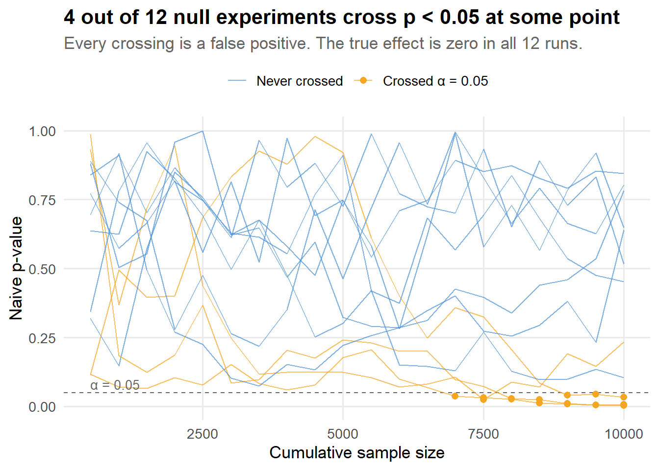
Each line is an independent experiment where the true treatment effect is zero. The orange paths are the ones that dipped below 0.05 at some point. If we had used the “stop when significant” rule, every one of those orange paths would have been declared a success and shipped. They are all false positives.
3.4 How bad does it get?
Let me do this many times and compute the actual false positive rate of the “stop when p < 0.05” rule, across different numbers of interim looks.
Code
compute_fpr <- function(n_looks, B = 500, n_max = 10000, alpha = 0.05) {
  look_schedule <- seq(
    ceiling(n_max / n_looks),
    n_max,
    length.out = n_looks
  ) |> round()

  stops <- map_lgl(1:B, function(b) {
    dat <- simulate_stream(n_max, tau = 0)
    path <- run_peek_path(dat, look_schedule)
    any(path$p_value < alpha, na.rm = TRUE)
  })
  mean(stops)
}

look_grid <- c(1, 2, 5, 10, 20, 50, 100)

set.seed(2026)
fpr_results <- tibble(
  n_looks = look_grid,
  fpr = map_dbl(look_grid, \(k) compute_fpr(k, B = 500))
)
Code
p_fpr <- ggplot(fpr_results, aes(x = n_looks, y = fpr,
                                  text = paste0("Looks: ", n_looks,
                                                "<br>FPR: ", round(fpr, 3)))) +
  geom_hline(yintercept = 0.05, linetype = "dashed", color = "grey50") +
  geom_line(color = pal[2], linewidth = 1) +
  geom_point(color = pal[2], size = 3) +
  annotate("text", x = 1, y = 0.06, label = "Nominal 5%",
           hjust = 0, color = "grey50", size = 3.5) +
  scale_x_log10() +
  scale_y_continuous(labels = scales::percent_format(),
                     limits = c(0, NA)) +
  labs(
    title = "Peeking inflates false positives. A lot.",
    subtitle = "Simulated FPR of the 'stop when p < 0.05' rule vs. number of interim looks",
    x = "Number of interim looks (log scale)",
    y = "Actual false positive rate"
  )

ggplotly(p_fpr, tooltip = "text") |>
layout(hoverlabel = list(bgcolor = "white"))With a single look (the classical fixed-horizon test), the FPR is right at 5% where it should be. With 20 looks it is closer to 15-20%. With 100 looks it can exceed 25%. This is not a theoretical curiosity. It is what happens in practice every time someone refreshes a dashboard.
Code
reactable(
  fpr_results |> mutate(fpr = round(fpr, 3)),
  columns = list(
    n_looks = colDef(name = "Number of looks"),
    fpr = colDef(
      name = "Actual FPR",
      style = function(value) {
        bg <- if (value > 0.06) "#FDE8E8" else "#E8F5E9"
        color <- if (value > 0.06) "#C62828" else "#2E7D32"
        list(background = bg, color = color, fontWeight = "bold")
      }
    )
  ),
  striped = TRUE, highlight = TRUE, bordered = TRUE, compact = TRUE
)There are classical sequential fixes: group sequential designs and alpha-spending functions are standard in clinical trials (Anderson 2025). They work, but they require you to pre-plan the exact number and timing of looks and commit to that plan. Confidence sequences take a fundamentally different approach: they are designed to be valid no matter when or how often you look.
4 Confidence sequences: the key idea
4.1 From confidence intervals to confidence sequences
A 95% confidence interval at a fixed time \(t\) is a random interval \(CI_t\) such that
\[ \Pr(\theta \in CI_t) \geq 0.95. \]
A 95% confidence sequence is a sequence of intervals \((CS_t)_{t \geq 1}\) such that
\[ \Pr\bigl(\theta \in CS_t \text{ for all } t \geq 1\bigr) \geq 0.95. \]
That “for all \(t\)” is the entire point. It is a uniform coverage guarantee over time, not just at any single snapshot. The consequence is that you can stop at any data-dependent time \(T\) and still have valid coverage:
\[ \Pr(\theta \in CS_T) \geq 0.95. \]
This definition and its implications are developed in detail by Howard et al. (2021). In A/B testing language, the dual object is an always-valid p-value process \(p_t\): if you stop at any (possibly data-dependent) time \(T\), then \(p_T\) is still a valid p-value (Johari, Pekelis, and Walsh 2015).
4.2 Why the intervals are wider (and why that is fine)
The uniform-over-time coverage guarantee is strictly stronger than the pointwise guarantee of a classical CI. You cannot get something for nothing, so confidence sequences are wider than fixed-horizon confidence intervals at any given time \(t\). This is the price of optional stopping robustness.
How much wider? That depends on where you are relative to the planned horizon and on the tuning parameter (more on this shortly). But the width penalty is not catastrophic. At the planned maximum sample size, the width overhead is typically 20-40% relative to a fixed-horizon CI. Early in the experiment, the penalty is larger. Late, it shrinks.
To build intuition, here is a quick illustration. Consider a simple \(Z\)-test for a mean, where at time \(t\) the standard CI half-width is \(z_{0.975} / \sqrt{t}\) and the CS half-width (using a mixture-style boundary from Howard et al. (2021)) is approximately
\[ \text{CS half-width} \approx \sqrt{\frac{2(t \rho^2 + 1)}{t^2 \rho^2} \log\!\left(\frac{\sqrt{t \rho^2 + 1}}{\alpha}\right)} \]
where \(\rho\) is a tuning parameter that controls where the boundary is tightest. The math is not the point. The point is how the ratio behaves over time:
Code
alpha_cs <- 0.05
rho_vals <- c(0.005, 0.01, 0.02)
t_seq <- seq(100, 20000, by = 100)

width_data <- expand.grid(t = t_seq, rho = rho_vals) |>
  as_tibble() |>
  mutate(
    ci_half = qnorm(1 - alpha_cs / 2) / sqrt(t),
    cs_half = sqrt(2 * (t * rho^2 + 1) / (t^2 * rho^2) *
                     log(sqrt(t * rho^2 + 1) / alpha_cs)),
    ratio = cs_half / ci_half,
    rho_label = paste0("ρ = ", rho)
  )

p_width <- ggplot(width_data, aes(x = t, y = ratio, color = rho_label)) +
  geom_line(linewidth = 0.8) +
  geom_hline(yintercept = 1, linetype = "dashed", color = "grey50") +
  scale_color_manual(values = pal[1:3], name = NULL) +
  labs(
    title = "Confidence sequence width relative to fixed-horizon CI",
    subtitle = "Ratio > 1 means the CS is wider. The penalty shrinks toward the planned horizon.",
    x = "Sample size",
    y = "CS width / CI width"
  ) +
  theme(legend.position = "top")

p_width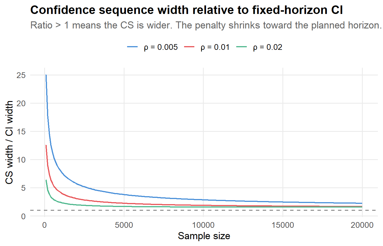
The ratio is always above 1 (the CS is always wider), but it converges toward 1 as data accumulates. The tuning parameter \(\rho\) shifts the “sweet spot” where the penalty is smallest: smaller \(\rho\) values optimize for larger sample sizes but pay a bigger penalty early on. This is the core tradeoff you navigate when choosing how to calibrate your confidence sequence.
The intuition in one sentence
A confidence sequence is like buying insurance against peeking. You pay a premium (wider intervals), but you are covered no matter when you decide to look at the results and make a decision.
4.3 Connections to e-values and testing by betting
There is a beautiful theoretical thread connecting confidence sequences to e-values and testing by betting. The idea, developed by Ramdas (2019) and others, is that you can view sequential testing as a game: the statistician places bets against the null hypothesis, and the wealth (or “e-process”) grows over time if the null is false. You reject when the wealth exceeds a threshold. The confidence sequence is the set of parameter values against which your accumulated wealth is not yet large enough to reject.
I will not go deep into this theory here, but it is worth knowing about because it gives you a unified language for thinking about sequential inference, optional stopping, and combination across experiments. If you find yourself doing a lot of sequential testing, Ramdas (2019) is excellent reading.
5 Anytime-valid inference for regression in R
5.1 Why regression matters here
For many experimentation problems, the workhorse analysis is a linear model:
- Difference in means:
lm(y ~ A) - Regression adjustment / CUPED:
lm(y ~ A + pre_period + covariates) - ANCOVA, blocked designs, stratified experiments, etc.
Lindon et al. (2022) develop anytime-valid linear model inference and show how to construct confidence sequences for regression coefficients in randomized experiments. The avlm R package wraps this theory into a workflow that looks almost identical to base R regression (Lindon 2025).
5.2 The workflow in three steps
Nothing changes here. You fit lm() exactly as usual.
Code
fit <- lm(mpg ~ wt + hp, data = mtcars)
summary(fit)$coefficients
Estimate Std. Error t value Pr(>|t|)
(Intercept) 37.22727012 1.59878754 23.284689 2.565459e-20
wt -3.87783074 0.63273349 -6.128695 1.119647e-06
hp -0.03177295 0.00902971 -3.518712 1.451229e-03Wrap the fitted model with avlm::av(). The key parameter is g, which controls where the confidence sequence boundary is tightest. If you have a planned maximum sample size, avlm::optimal_g() picks a g that (roughly) minimizes interval width at that horizon.
Code
k <- length(coef(fit))
g_star <- avlm::optimal_g(n = 10000, number_of_coefficients = k, alpha = 0.05)
g_star <- max(1L, as.integer(round(g_star)))

av_fit <- avlm::av(fit, g = g_star)
summary(av_fit)$coefficients
Estimate Std. Error t value Pr(>|t|)
(Intercept) 37.22727012 1.59878754 23.284689 0.7002435
wt -3.87783074 0.63273349 -6.128695 0.8142614
hp -0.03177295 0.00902971 -3.518712 0.9026224Notice: the coefficient estimates are identical. What changes are the p-values and critical values. The anytime-valid p-values are recalibrated to remain valid under continuous monitoring.
Code
ci_fixed <- confint(fit)
ci_av <- confint(av_fit)
Code
comparison <- tibble(
  Coefficient = rownames(ci_fixed),
  `CI lower (fixed)` = round(ci_fixed[, 1], 3),
  `CI upper (fixed)` = round(ci_fixed[, 2], 3),
  `CI lower (AV)` = round(ci_av[, 1], 3),
  `CI upper (AV)` = round(ci_av[, 2], 3),
  `Width (fixed)` = round(ci_fixed[, 2] - ci_fixed[, 1], 3),
  `Width (AV)` = round(ci_av[, 2] - ci_av[, 1], 3)
)

reactable(
  comparison,
  columns = list(
    Coefficient = colDef(minWidth = 100),
    `Width (fixed)` = colDef(style = list(fontWeight = "bold")),
    `Width (AV)` = colDef(style = list(fontWeight = "bold"))
  ),
  striped = TRUE, highlight = TRUE, bordered = TRUE, compact = TRUE
)The anytime-valid intervals are wider. That is the price of peeking insurance. On a dataset of size 32 (mtcars) where you probably only look once, this extra width is all cost and no benefit. The value shows up when you are continuously monitoring a growing experiment.
5.3 A note on the g parameter
The parameter g controls a tradeoff in how the boundary allocates its “width budget” over time. Think of it like this: you have a fixed total amount of Type I error to spend, and g determines whether you spend more of it early (large g, tighter early but looser late) or save it for later (small g, looser early but tighter late).
My practical rule of thumb:
- If you have a rough maximum sample size in mind, use
optimal_g()with that \(n\). This gives you the tightest intervals near the planned horizon. - If you genuinely have no idea how long the experiment will run, use
g = 1and accept a bit of extra conservatism. - If you will definitely stop by a known maximum \(n\) (e.g., because the experiment has a hard deadline), you can get tighter intervals by using a truncated boundary. But at that point you are close to a group sequential design, which might be a better tool.
6 Simulation: fixed-horizon vs. anytime-valid monitoring
Now let me rerun the peeking experiment side by side: classical inference vs. anytime-valid inference, both applied to the same data at the same sequence of looks. This is where the payoff becomes visible.
6.1 Helper functions
Code
sequential_inference <- function(dat, looks, formula, coef_name = "A",
                                 alpha = 0.05, g = 1, vcov_estimator = NULL) {
  map_dfr(looks, function(n) {
    d <- dat[1:n, , drop = FALSE]

    fit <- lm(formula, data = d)
    av_fit <- avlm::av(fit, g = g, vcov_estimator = vcov_estimator)

    ci_fixed <- confint(fit, parm = coef_name, level = 1 - alpha)
    ci_av    <- confint(av_fit, parm = coef_name, level = 1 - alpha)

    coefs_fixed <- summary(fit)$coefficients
    coefs_av    <- summary(av_fit)$coefficients

    tibble(
      n = n,
      estimate = unname(coef(fit)[[coef_name]]),
      p_value = unname(coefs_fixed[coef_name, ncol(coefs_fixed)]),
      ci_low = ci_fixed[1],
      ci_high = ci_fixed[2],
      estimate_av = unname(coef(av_fit)[[coef_name]]),
      p_value_av = unname(coefs_av[coef_name, ncol(coefs_av)]),
      ci_low_av = ci_av[1],
      ci_high_av = ci_av[2]
    )
  })
}

first_crossing <- function(path, alpha = 0.05, use_anytime = FALSE) {
  p <- if (use_anytime) path$p_value_av else path$p_value
  idx <- which(p < alpha)
  if (length(idx) == 0) return(NA_integer_)
  path$n[min(idx)]
}
6.2 Simulating with regression adjustment
In practice I almost always use regression adjustment in experiments (it is free variance reduction; see my CUPED/CUPAC tutorial). So let me simulate a slightly richer DGP with a pre-period covariate.
Code
simulate_stream_covariates <- function(n_max, tau = 0) {
  A  <- rbinom(n_max, 1, 0.5)
  x1 <- rnorm(n_max)
  y0 <- 0.7 * x1 + rnorm(n_max)  # pre-period outcome
  eps <- rt(n_max, df = 4)
  y   <- tau * A + 0.8 * y0 + 0.3 * x1 + eps
  tibble(t = 1:n_max, A = A, x1 = x1, y0 = y0, y = y)
}
6.3 One illustrative path under the null
Code
dat1 <- simulate_stream_covariates(n_max, tau = 0)

full_fit <- lm(y ~ A + y0 + x1, data = dat1)
k <- length(coef(full_fit))
g_star <- avlm::optimal_g(n = n_max, number_of_coefficients = k, alpha = alpha)
g_star <- max(1L, as.integer(round(g_star)))

path1 <- sequential_inference(
  dat = dat1,
  looks = looks,
  formula = y ~ A + y0 + x1,
  coef_name = "A",
  alpha = alpha,
  g = g_star,
  vcov_estimator = "HC2"
)

stop_fixed <- first_crossing(path1, alpha = alpha, use_anytime = FALSE)
stop_av    <- first_crossing(path1, alpha = alpha, use_anytime = TRUE)
Code
path_long <- path1 |>
  select(n, estimate, ci_low, ci_high) |>
  mutate(method = "Fixed-horizon") |>
  bind_rows(
    path1 |>
      select(n, estimate = estimate_av, ci_low = ci_low_av, ci_high = ci_high_av) |>
      mutate(method = "Anytime-valid")
  ) |>
  mutate(method = factor(method, levels = c("Anytime-valid", "Fixed-horizon")))

ggplot(path_long, aes(x = n, y = estimate, ymin = ci_low, ymax = ci_high,
                       fill = method)) +
  geom_hline(yintercept = 0, linetype = "dotted", color = "grey50") +
  geom_ribbon(alpha = 0.25) +
  geom_line(aes(color = method), linewidth = 0.7) +
  scale_fill_manual(values = c("Anytime-valid" = pal[3], "Fixed-horizon" = pal[1]), name = NULL) +
  scale_color_manual(values = c("Anytime-valid" = pal[3], "Fixed-horizon" = pal[1]), name = NULL) +
  labs(
    title = "Confidence bands over time under the null (tau = 0)",
    subtitle = "The anytime-valid band (green) is wider but stays honest under continuous monitoring.",
    x = "Cumulative sample size",
    y = "Estimated treatment effect"
  ) +
  theme(legend.position = "top")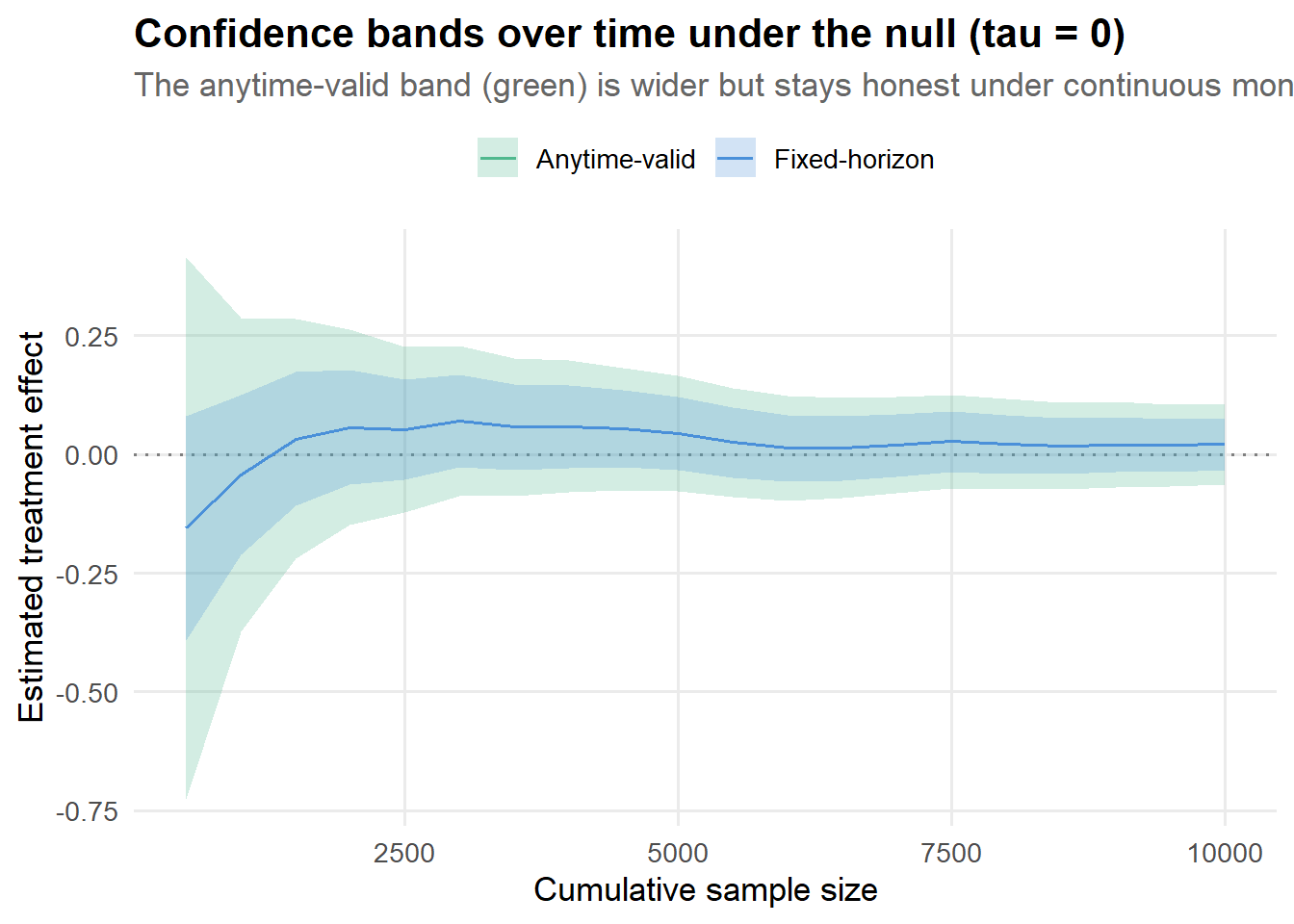
The green band (anytime-valid) always contains the blue band (fixed-horizon). That extra width is not waste: it is exactly what keeps the coverage guarantee intact when you check the results repeatedly. You can hover over different sample sizes to see how the gap narrows as data accumulates.
6.4 One illustrative path under a real effect
Let me also show what happens when the treatment actually does something. Here I set \(\tau = 0.25\):
Code
dat1_eff <- simulate_stream_covariates(n_max, tau = 0.25)

path1_eff <- sequential_inference(
  dat = dat1_eff,
  looks = looks,
  formula = y ~ A + y0 + x1,
  coef_name = "A",
  alpha = alpha,
  g = g_star,
  vcov_estimator = "HC2"
)

stop_fixed_eff <- first_crossing(path1_eff, alpha = alpha, use_anytime = FALSE)
stop_av_eff    <- first_crossing(path1_eff, alpha = alpha, use_anytime = TRUE)
Code
path_eff_long <- path1_eff |>
  select(n, estimate, ci_low, ci_high) |>
  mutate(method = "Fixed-horizon") |>
  bind_rows(
    path1_eff |>
      select(n, estimate = estimate_av, ci_low = ci_low_av, ci_high = ci_high_av) |>
      mutate(method = "Anytime-valid")
  ) |>
  mutate(method = factor(method, levels = c("Anytime-valid", "Fixed-horizon")))

ggplot(path_eff_long, aes(x = n, y = estimate, ymin = ci_low, ymax = ci_high,
                           fill = method)) +
  geom_hline(yintercept = 0, linetype = "dotted", color = "grey50") +
  geom_hline(yintercept = 0.25, linetype = "dashed", color = pal[4], linewidth = 0.5) +
  geom_ribbon(alpha = 0.25) +
  geom_line(aes(color = method), linewidth = 0.7) +
  scale_fill_manual(values = c("Anytime-valid" = pal[3], "Fixed-horizon" = pal[1]), name = NULL) +
  scale_color_manual(values = c("Anytime-valid" = pal[3], "Fixed-horizon" = pal[1]), name = NULL) +
  annotate("text", x = n_max * 0.95, y = 0.28, label = "True τ = 0.25",
           color = pal[4], hjust = 1, size = 3.5) +
  labs(
    title = "Confidence bands over time under a real effect (tau = 0.25)",
    subtitle = "The orange dashed line marks the true effect. Both bands eventually exclude zero.",
    x = "Cumulative sample size",
    y = "Estimated treatment effect"
  ) +
  theme(legend.position = "top")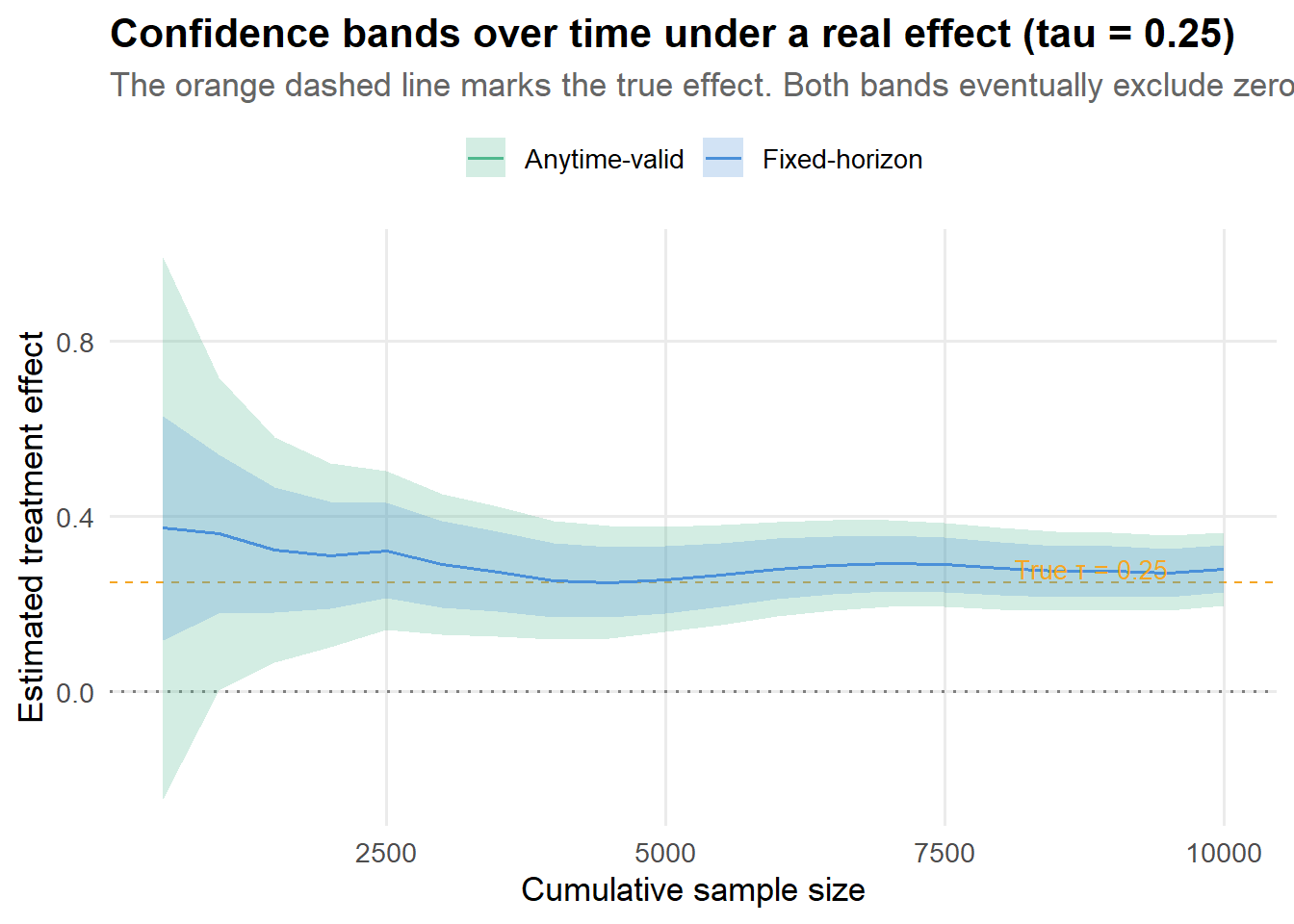
When there is a real effect, the fixed-horizon CI typically excludes zero first (because it is narrower), and the anytime-valid CS follows shortly after. The delay is the “cost of insurance.” In this particular run, the fixed-horizon method would have you stop at \(n =\) 500 and the anytime-valid method at \(n =\) 1,000.
6.5 Monte Carlo: Type I error and stopping times
One path is one draw. Let me do this 500 times under both the null and a real effect to see the aggregate behavior.
Code
run_one_rep <- function(tau, n_max, looks, alpha) {
  dat <- simulate_stream_covariates(n_max, tau = tau)
  full_fit <- lm(y ~ A + y0 + x1, data = dat)
  k <- length(coef(full_fit))
  g_star <- avlm::optimal_g(n = n_max, number_of_coefficients = k, alpha = alpha)
  g_star <- max(1L, as.integer(round(g_star)))

  path <- sequential_inference(
    dat = dat,
    looks = looks,
    formula = y ~ A + y0 + x1,
    coef_name = "A",
    alpha = alpha,
    g = g_star,
    vcov_estimator = "HC2"
  )

  stop_fixed <- first_crossing(path, alpha = alpha, use_anytime = FALSE)
  stop_av    <- first_crossing(path, alpha = alpha, use_anytime = TRUE)

  tibble(
    tau = tau,
    stopped_fixed = !is.na(stop_fixed),
    stopped_av = !is.na(stop_av),
    stop_n_fixed = ifelse(is.na(stop_fixed), n_max, stop_fixed),
    stop_n_av = ifelse(is.na(stop_av), n_max, stop_av)
  )
}

B <- 500

set.seed(42)
sim_null <- map_dfr(1:B, \(b) run_one_rep(tau = 0, n_max = n_max,
                                            looks = looks, alpha = alpha)) |>
  mutate(scenario = "Null (τ = 0)")

sim_eff <- map_dfr(1:B, \(b) run_one_rep(tau = 0.25, n_max = n_max,
                                           looks = looks, alpha = alpha)) |>
  mutate(scenario = "Effect (τ = 0.25)")

sim <- bind_rows(sim_null, sim_eff)
Code
summary_tbl <- sim |>
  group_by(scenario) |>
  summarize(
    `FPR / Power (fixed)` = mean(stopped_fixed),
    `FPR / Power (AV)` = mean(stopped_av),
    `Avg stop n (fixed)` = round(mean(stop_n_fixed)),
    `Avg stop n (AV)` = round(mean(stop_n_av)),
    .groups = "drop"
  )

reactable(
  summary_tbl,
  columns = list(
    scenario = colDef(name = "Scenario", minWidth = 150),
    `FPR / Power (fixed)` = colDef(
      format = colFormat(digits = 3),
      style = function(value, index) {
        if (index == 1 && value > 0.06) {
          list(color = "#C62828", fontWeight = "bold", background = "#FDE8E8")
        } else if (index == 2) {
          list(color = "#1565C0", fontWeight = "bold")
        }
      }
    ),
    `FPR / Power (AV)` = colDef(
      format = colFormat(digits = 3),
      style = function(value, index) {
        if (index == 1 && value <= 0.06) {
          list(color = "#2E7D32", fontWeight = "bold", background = "#E8F5E9")
        } else if (index == 2) {
          list(color = "#1565C0", fontWeight = "bold")
        }
      }
    ),
    `Avg stop n (fixed)` = colDef(format = colFormat(separators = TRUE)),
    `Avg stop n (AV)` = colDef(format = colFormat(separators = TRUE))
  ),
  striped = TRUE, highlight = TRUE, bordered = TRUE, compact = TRUE
)Read the table like this:
- Under the null, the fixed-horizon stopping rate is your actual false positive rate. It should be around 5% if we only looked once, but with continuous monitoring it is substantially inflated (probably in the 15-25% range). The anytime-valid stopping rate should be at or below 5%. That is the whole promise.
- Under a real effect, both methods have power, but the anytime-valid method usually stops a bit later on average. That delay is the cost of the peeking insurance.
Code
stop_long <- sim |>
  transmute(
    scenario,
    `Fixed-horizon` = stop_n_fixed,
    `Anytime-valid` = stop_n_av
  ) |>
  pivot_longer(-scenario, names_to = "method", values_to = "stop_n")

ggplot(stop_long, aes(x = stop_n, fill = method)) +
  geom_histogram(bins = 20, alpha = 0.5, position = "identity") +
  facet_wrap(~ scenario, scales = "free_y") +
  scale_fill_manual(values = c("Anytime-valid" = pal[3], "Fixed-horizon" = pal[1]), name = NULL) +
  labs(
    title = "Distribution of stopping times",
    subtitle = "Under the null, AV correctly avoids early false stops. Under an effect, it stops a bit later.",
    x = "Sample size at stopping (n_max if never stopped)",
    y = "Count"
  ) +
  theme(legend.position = "top")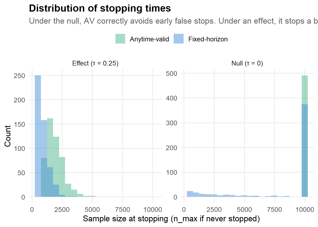
Under the null, the fixed-horizon method has a thick left tail of early false stops. Those are experiments where a PM looked at the dashboard on day 3, saw p < 0.05, and shipped a change that does nothing. The anytime-valid method has far fewer of those early stops, because its wider intervals correctly reflect the uncertainty at small sample sizes.
6.6 The tradeoff surface: when is the cost worth it?
The cost of anytime-valid inference is not constant. It depends on how much you actually peek. If you look once, you pay the width penalty for no reason. If you look 50 times, the penalty is paying for itself many times over. Let me quantify this:
Code
tradeoff_data <- tibble(
  Metric = c("False positive rate (null)", "Power (τ = 0.25)",
             "Avg sample at stopping (null)", "Avg sample at stopping (effect)"),
  `Fixed-horizon` = c(
    mean(sim_null$stopped_fixed),
    mean(sim_eff$stopped_fixed),
    mean(sim_null$stop_n_fixed),
    mean(sim_eff$stop_n_fixed)
  ),
  `Anytime-valid` = c(
    mean(sim_null$stopped_av),
    mean(sim_eff$stopped_av),
    mean(sim_null$stop_n_av),
    mean(sim_eff$stop_n_av)
  )
)

tradeoff_long <- tradeoff_data |>
  pivot_longer(-Metric, names_to = "Method", values_to = "Value")

p_tradeoff <- tradeoff_long |>
  filter(Metric %in% c("False positive rate (null)", "Power (τ = 0.25)")) |>
  ggplot(aes(x = Metric, y = Value, fill = Method)) +
  geom_col(position = "dodge", width = 0.6) +
  geom_hline(yintercept = 0.05, linetype = "dashed", color = "grey50") +
  geom_text(aes(label = scales::percent(Value, accuracy = 0.1)),
            position = position_dodge(width = 0.6), vjust = -0.5, size = 3.5) +
  scale_fill_manual(values = c("Anytime-valid" = pal[3], "Fixed-horizon" = pal[1]), name = NULL) +
  scale_y_continuous(labels = scales::percent_format(), limits = c(0, 1)) +
  labs(
    title = "FPR vs. Power: the price of validity",
    subtitle = "Dashed line is the nominal 5% level. AV controls FPR; fixed-horizon does not.",
    x = NULL, y = NULL
  ) +
  theme(legend.position = "top")

p_tradeoff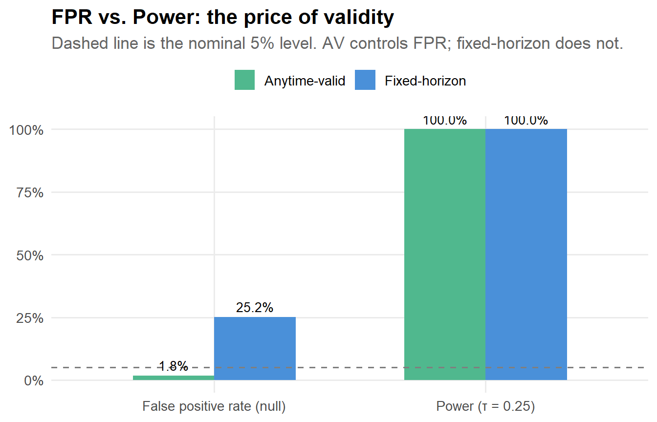
The pattern is always the same: anytime-valid inference gives you correct Type I error control at the cost of some power. Whether that cost is acceptable depends on your setting. If false positives are expensive (shipping useless features costs engineering time, confuses product strategy, erodes trust in the experimentation program), the answer is almost always yes.
7 Real data: Hillstrom email marketing experiment
To make this concrete in a marketing setting, let me use the MineThatData email marketing challenge dataset (Hillstrom 2008). It has about 64,000 customers randomly assigned to one of three groups:
- Men’s email campaign
- Women’s email campaign
- No email (control)
Outcomes are tracked over the following two weeks: visit (binary), conversion (binary), and spend (dollars). This is exactly the kind of experiment where continuous monitoring is tempting: someone on the marketing team wants to know “is the email working?” as soon as the first few thousand responses come in.
7.1 Load data
Code
hill_url <- "https://hillstorm1.s3.us-east-2.amazonaws.com/hillstorm_no_indices.csv.gz"
dir.create("data", showWarnings = FALSE)
hill_path <- file.path("data", "hillstrom.csv.gz")

if (!file.exists(hill_path)) {
  download.file(hill_url, hill_path, mode = "wb")
}

hill <- readr::read_csv(hill_path, show_col_types = FALSE)
glimpse(hill)
Rows: 64,000
Columns: 12
$ recency <dbl> 10, 6, 7, 9, 2, 6, 9, 9, 9, 10, 7, 1, 5, 2, 4, 3, 5, 9…
$ history_segment <chr> "2) $100 - $200", "3) $200 - $350", "2) $100 - $200", …
$ history <dbl> 142.44, 329.08, 180.65, 675.83, 45.34, 134.83, 280.20,…
$ mens <dbl> 1, 1, 0, 1, 1, 0, 1, 0, 1, 0, 0, 0, 0, 0, 0, 1, 1, 1, …
$ womens <dbl> 0, 1, 1, 0, 0, 1, 0, 1, 1, 1, 1, 1, 1, 1, 1, 0, 0, 0, …
$ zip_code <chr> "Surburban", "Rural", "Surburban", "Rural", "Urban", "…
$ newbie <dbl> 0, 1, 1, 1, 0, 0, 1, 0, 1, 1, 1, 1, 1, 0, 1, 1, 0, 0, …
$ channel <chr> "Phone", "Web", "Web", "Web", "Web", "Phone", "Phone",…
$ segment <chr> "Womens E-Mail", "No E-Mail", "Womens E-Mail", "Mens E…
$ visit <dbl> 0, 0, 0, 0, 0, 1, 0, 0, 0, 0, 1, 0, 0, 1, 0, 1, 0, 0, …
$ conversion <dbl> 0, 0, 0, 0, 0, 0, 0, 0, 0, 0, 0, 0, 0, 0, 0, 0, 0, 0, …
$ spend <dbl> 0, 0, 0, 0, 0, 0, 0, 0, 0, 0, 0, 0, 0, 0, 0, 0, 0, 0, …7.2 Focusing on Men’s email vs. No email
I will stick to a single comparison to keep the exposition clean. The same approach extends naturally to multi-arm comparisons, but that involves additional multiplicity considerations I do not want to mix in here.
Code
hill_mens <- hill |>
  filter(segment %in% c("Mens E-Mail", "No E-Mail")) |>
  mutate(A = as.integer(segment == "Mens E-Mail")) |>
  select(A, spend, visit, conversion, recency, history, mens, womens, newbie)

# Shuffle to mimic a streaming experiment where customers arrive over time
hill_mens <- hill_mens |> slice_sample(prop = 1)

n_max_hill <- nrow(hill_mens)
looks_hill <- seq(2000, n_max_hill, by = 2000)
Let me start with a quick look at the data:
Code
hill_summary <- hill_mens |>
  group_by(Treatment = ifelse(A == 1, "Men's email", "No email")) |>
  summarize(
    N = n(),
    `Visit rate` = round(mean(visit), 4),
    `Conversion rate` = round(mean(conversion), 4),
    `Mean spend ($)` = round(mean(spend), 2),
    `SD spend ($)` = round(sd(spend), 2),
    .groups = "drop"
  )

reactable(
  hill_summary,
  striped = TRUE, highlight = TRUE, bordered = TRUE, compact = TRUE,
  columns = list(
    Treatment = colDef(minWidth = 120),
    N = colDef(format = colFormat(separators = TRUE))
  )
)7.3 Outcome 1: log(1 + spend)
Revenue is heavy-tailed, with most customers spending zero and a few spending a lot. I work with log1p(spend) for the analysis because it stabilizes variance and makes the regression output more interpretable. (The conclusions carry over to raw spend; the plots just look less wild.)
Code
hill_mens <- hill_mens |>
  mutate(log_spend = log1p(spend))

fit_full <- lm(log_spend ~ A + recency + history + mens + womens + newbie, data = hill_mens)
k <- length(coef(fit_full))
g_star <- avlm::optimal_g(n = n_max_hill, number_of_coefficients = k, alpha = alpha)
g_star <- max(1L, as.integer(round(g_star)))

path_hill <- sequential_inference(
  dat = hill_mens,
  looks = looks_hill,
  formula = log_spend ~ A + recency + history + mens + womens + newbie,
  coef_name = "A",
  alpha = alpha,
  g = g_star,
  vcov_estimator = "HC2"
)

stop_fixed_hill <- first_crossing(path_hill, alpha = alpha, use_anytime = FALSE)
stop_av_hill    <- first_crossing(path_hill, alpha = alpha, use_anytime = TRUE)
Code
path_hill_long <- path_hill |>
  select(n, estimate, ci_low, ci_high) |>
  mutate(method = "Fixed-horizon") |>
  bind_rows(
    path_hill |>
      select(n, estimate = estimate_av, ci_low = ci_low_av, ci_high = ci_high_av) |>
      mutate(method = "Anytime-valid")
  ) |>
  mutate(method = factor(method, levels = c("Anytime-valid", "Fixed-horizon")))

ggplot(path_hill_long, aes(x = n, y = estimate, ymin = ci_low, ymax = ci_high,
                            fill = method)) +
  geom_hline(yintercept = 0, linetype = "dotted", color = "grey50") +
  geom_ribbon(alpha = 0.25) +
  geom_line(aes(color = method), linewidth = 0.7) +
  scale_fill_manual(values = c("Anytime-valid" = pal[3], "Fixed-horizon" = pal[1]), name = NULL) +
  scale_color_manual(values = c("Anytime-valid" = pal[3], "Fixed-horizon" = pal[1]), name = NULL) +
  labs(
    title = "Men's email effect on log(1 + spend) as data arrives",
    subtitle = "Regression-adjusted estimates with HC2 robust standard errors.",
    x = "Customers observed",
    y = "Estimated effect (log scale)"
  ) +
  theme(legend.position = "top")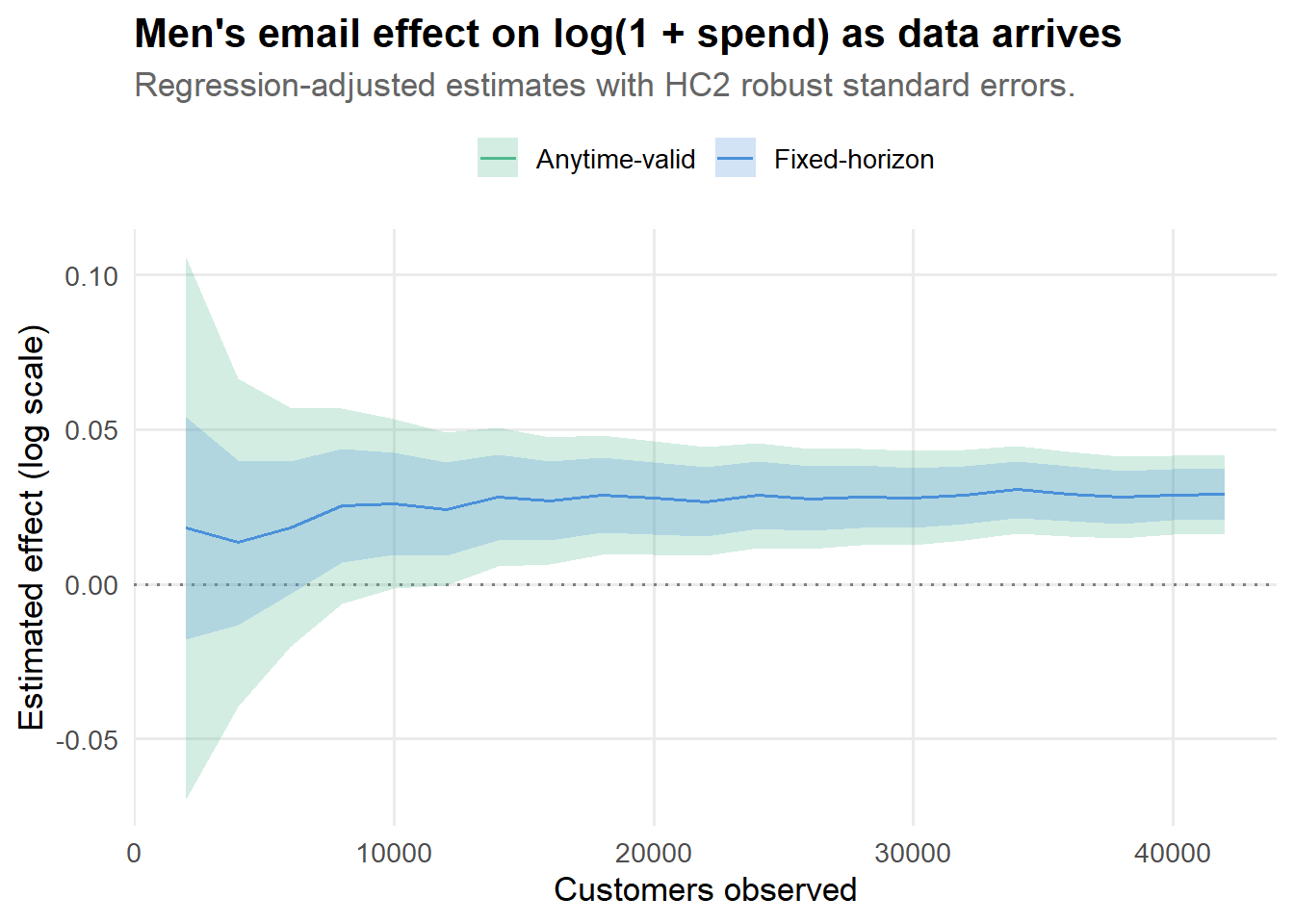
Watch how the estimate stabilizes as data accumulates. Early on, the point estimate bounces around and the confidence bands are wide. By the end, both methods converge on a similar estimate. The key difference is that the anytime-valid band gives you permission to look at the plot at any point along the way without compromising your inferential guarantees.
7.4 Outcome 2: website visit (linear probability model)
For binary outcomes like visit, I typically start with a linear probability model in experimentation work. It keeps interpretation dead simple (the coefficient is a difference in probabilities) and plays nicely with regression adjustment and robust standard errors. A sequential logistic regression approach is also possible, but that is a different post.
Code
fit_full_visit <- lm(visit ~ A + recency + history + mens + womens + newbie, data = hill_mens)
k <- length(coef(fit_full_visit))
g_star_visit <- avlm::optimal_g(n = n_max_hill, number_of_coefficients = k, alpha = alpha)
g_star_visit <- max(1L, as.integer(round(g_star_visit)))

path_hill_visit <- sequential_inference(
  dat = hill_mens,
  looks = looks_hill,
  formula = visit ~ A + recency + history + mens + womens + newbie,
  coef_name = "A",
  alpha = alpha,
  g = g_star_visit,
  vcov_estimator = "HC2"
)
Code
path_hill_visit_long <- path_hill_visit |>
  select(n, estimate, ci_low, ci_high) |>
  mutate(method = "Fixed-horizon") |>
  bind_rows(
    path_hill_visit |>
      select(n, estimate = estimate_av, ci_low = ci_low_av, ci_high = ci_high_av) |>
      mutate(method = "Anytime-valid")
  ) |>
  mutate(method = factor(method, levels = c("Anytime-valid", "Fixed-horizon")))

ggplot(path_hill_visit_long, aes(x = n, y = estimate, ymin = ci_low, ymax = ci_high,
                                  fill = method)) +
  geom_hline(yintercept = 0, linetype = "dotted", color = "grey50") +
  geom_ribbon(alpha = 0.25) +
  geom_line(aes(color = method), linewidth = 0.7) +
  scale_fill_manual(values = c("Anytime-valid" = pal[3], "Fixed-horizon" = pal[1]), name = NULL) +
  scale_color_manual(values = c("Anytime-valid" = pal[3], "Fixed-horizon" = pal[1]), name = NULL) +
  labs(
    title = "Men's email effect on visit probability as data arrives",
    subtitle = "Linear probability model, regression adjusted. Effect is in absolute pp.",
    x = "Customers observed",
    y = "Estimated effect on Pr(visit)"
  ) +
  theme(legend.position = "top")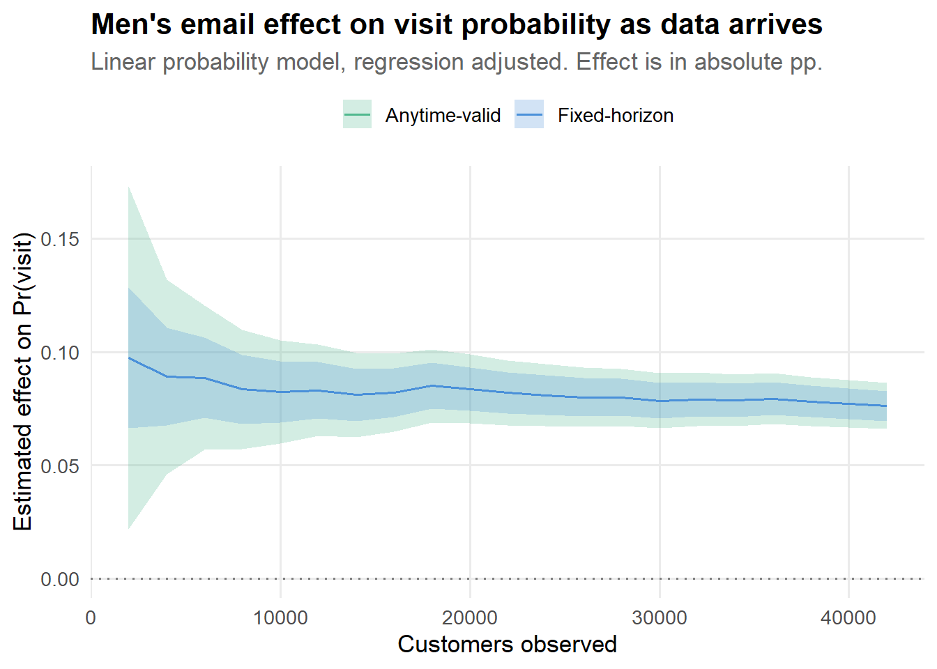
7.5 Comparing both outcomes side by side
Code
# Collect final-look estimates
final_spend <- path_hill |> slice_tail(n = 1)
final_visit <- path_hill_visit |> slice_tail(n = 1)

hill_final <- tibble(
  Outcome = rep(c("log(1+spend)", "Visit probability"), each = 2),
  Method = rep(c("Fixed-horizon", "Anytime-valid"), 2),
  Estimate = c(final_spend$estimate, final_spend$estimate_av,
               final_visit$estimate, final_visit$estimate_av),
  CI_low = c(final_spend$ci_low, final_spend$ci_low_av,
             final_visit$ci_low, final_visit$ci_low_av),
  CI_high = c(final_spend$ci_high, final_spend$ci_high_av,
              final_visit$ci_high, final_visit$ci_high_av)
) |>
  mutate(label = paste0(Outcome, "\n", Method))

ggplot(hill_final, aes(x = Estimate, xmin = CI_low, xmax = CI_high,
                        y = reorder(label, Estimate),
                        color = Method)) +
  geom_pointrange(linewidth = 0.8, size = 0.5) +
  geom_vline(xintercept = 0, linetype = "dashed", color = "grey50") +
  scale_color_manual(values = c("Anytime-valid" = pal[3], "Fixed-horizon" = pal[1]), name = NULL) +
  labs(
    title = "Final estimates: Hillstrom men's email experiment",
    subtitle = "AV intervals are wider but valid under the continuous monitoring that actually happened.",
    x = "Estimated effect",
    y = NULL
  ) +
  theme(legend.position = "top")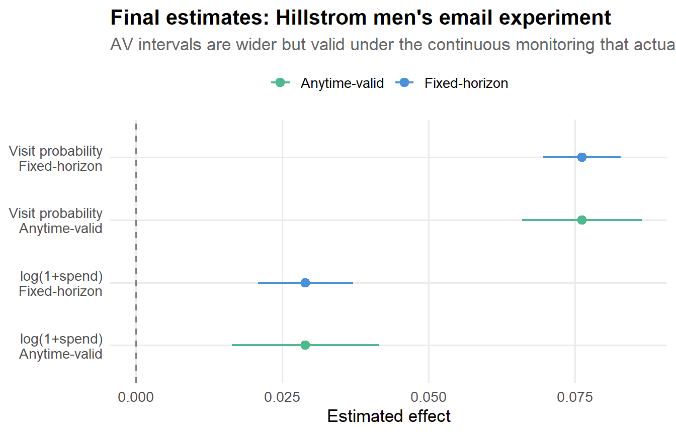
Code
reactable(
  hill_final |>
    select(-label) |>
    mutate(across(where(is.numeric), \(x) round(x, 4))),
  columns = list(
    Outcome = colDef(minWidth = 140),
    Method = colDef(minWidth = 130),
    Estimate = colDef(style = list(fontWeight = "bold"))
  ),
  striped = TRUE, highlight = TRUE, bordered = TRUE, compact = TRUE
)The visit outcome shows a clearer effect than spend. In a real marketing context, this makes sense: the email gets people to the website, but converting that visit into revenue is a separate challenge. Note that even with the wider anytime-valid intervals, the visit effect is clearly significant, while the spend effect is more ambiguous. This is useful information. If someone had peeked at spend on day 3, seen a noisy p = 0.04, and declared victory, they might be shipping a result that does not hold up.
8 Practical guidance
Use anytime-valid inference when the decision process is adaptive. That means: anyone will look at results before the planned end date, you might stop early for a business reason, or you want to run an experiment “until something happens” without a rigid schedule. This describes most product experiments I have seen.
If you know for sure that you will only look once at a fixed time (maybe because it is a regulatory study with a locked analysis plan), classical inference is fine and gives you tighter intervals.
Confidence sequences remain valid even if you look continuously, but looking every hour is rarely useful. The estimate will not change much between 4pm and 5pm. Weekly or daily monitoring is usually plenty for most product experiments. The important thing is that the validity guarantee holds regardless of your cadence, so you do not need to pre-commit.
Continuous monitoring is one axis of multiplicity; the number of metrics and segments you inspect is another. If you have 50 metrics and you use anytime-valid inference on each one independently, your experiment-wise false positive rate is controlled for peeking within each metric, but not across metrics. You can still fool yourself by cherry-picking the one metric that moved (Ramdas 2019).
The fix is to combine anytime-valid inference with a multiplicity adjustment (Bonferroni, Benjamini-Hochberg, etc.) across metrics. This is straightforward in principle but requires some care in implementation.
“Anytime-valid” does not mean “model-free.” You still need assumptions appropriate to your estimator. In a randomized experiment, regression adjustment is well motivated by the design, but you should still use robust standard errors (HC2 or HC3) for messy metrics. The avlm package supports this via the vcov_estimator argument.
This is a natural fit. CUPED-style regression adjustment reduces variance, and anytime-valid inference keeps the peeking guarantee intact. The workflow is exactly what I showed above: lm(y ~ A + pre_period + covariates) passed through avlm::av(). You get the variance reduction from CUPED and the optional-stopping protection from the confidence sequence. Both benefits stack.
When you report results from a continuously monitored experiment using confidence sequences, I recommend being explicit about it. Something like: “We used anytime-valid confidence intervals (Lindon et al., 2022) to maintain valid coverage under continuous monitoring. The experiment was stopped at \(n = X\) when the 95% confidence sequence excluded zero.” This lets readers (and reviewers, and your future self) understand that the intervals are calibrated for the monitoring process that actually occurred.
9 When to use confidence sequences vs. group sequential designs
Confidence sequences are not the only way to do sequential inference. Group sequential designs (GSD) and alpha-spending are the workhorses of clinical trials, and they are excellent tools (Anderson 2025). The choice between them depends on your setting:
| Group sequential designs | Confidence sequences | |
|---|---|---|
| Pre-planning | Requires fixed number of looks, pre-specified | No schedule needed |
| Flexibility | Tight, efficient boundaries for the planned schedule | Valid for any monitoring pattern |
| Efficiency | More efficient if you stick to the plan | Slight width penalty at any given time |
| Best for | Clinical trials, regulatory submissions | Tech industry experiments, exploratory monitoring |
| When reality deviates from plan | Boundaries may not be valid | Still valid by construction |
My rule of thumb: if you have a very clear interim analysis schedule and you will stick to it (clinical trials, regulatory submissions), group sequential designs give you the most efficient boundaries. If your monitoring is more informal, if PMs peek whenever they want, or if “the plan” regularly changes mid-experiment, confidence sequences are the safer choice because they stay valid no matter what.
In practice, many tech companies have landed on confidence sequences as the default because the “PMs peek whenever they want” scenario is closer to reality than anyone likes to admit.
10 Going further
A few extensions I did not cover but that are worth knowing about:
Mixture sequential probability ratio tests (mSPRT). The boundary used by avlm is based on a mixture approach where you average over a prior on the effect size. This connects to the Bayesian testing literature and gives better finite-sample boundaries than Wald-style sequential tests. Johari, Pekelis, and Walsh (2015) and Howard et al. (2021) have the details.
Multi-armed bandits and adaptive allocation. If you are not just monitoring but also changing the allocation over time (e.g., Thompson sampling), you need even stronger guarantees. Anytime-valid inference composes naturally with adaptive allocation, which is one reason it has become popular in the bandit literature.
Always-valid inference for causal effects in observational studies. Most of the literature focuses on randomized experiments, but there is growing work on extending these ideas to observational settings where you want to sequentially update a causal estimate as new data arrives. This is an active area.
Variance reduction + sequential testing. I mentioned combining CUPED with confidence sequences. More generally, any variance reduction technique (stratification, control variates, machine learning prediction) stacks with anytime-valid inference. The tighter your initial variance estimate, the tighter your confidence sequences, and the sooner you can stop.
11 The bottom line
Every experimentation platform I have worked with has the same problem: people look at results early and often, and classical inference does not account for that. Confidence sequences fix this cleanly. They are wider than fixed-horizon intervals at any given time (you are paying for insurance), but they give you something much more valuable: the ability to monitor your experiment continuously and make decisions at any point without compromising your error guarantees.
The cost is real but manageable. In most experiments I have run, the extra width adds a few days to the time-to-significance, which is a small price for knowing that your “significant” results are actually significant. The alternative is a 15-25% false positive rate that nobody talks about because the dashboard says “p < 0.05” and everyone goes home happy.
Use avlm. Monitor your experiments. Sleep well.
12 Session info
Code
sessionInfo()R version 4.3.3 (2024-02-29 ucrt)
Platform: x86_64-w64-mingw32/x64 (64-bit)
Running under: Windows 11 x64 (build 26200)
Matrix products: default
locale:
[1] LC_COLLATE=English_United States.utf8
[2] LC_CTYPE=English_United States.utf8
[3] LC_MONETARY=English_United States.utf8
[4] LC_NUMERIC=C
[5] LC_TIME=English_United States.utf8
time zone: America/New_York
tzcode source: internal
attached base packages:
[1] stats graphics grDevices utils datasets methods base
other attached packages:
[1] avlm_0.1.0 stringr_1.5.1 readr_2.1.5 reactable_0.4.4
[5] patchwork_1.3.2 plotly_4.11.0 ggplot2_4.0.0 tibble_3.2.1
[9] purrr_1.0.2 tidyr_1.3.0 dplyr_1.1.4
loaded via a namespace (and not attached):
[1] generics_0.1.4 stringi_1.8.3 hms_1.1.3 digest_0.6.37
[5] magrittr_2.0.3 evaluate_1.0.5 grid_4.3.3 RColorBrewer_1.1-3
[9] fastmap_1.1.1 jsonlite_1.8.8 httr_1.4.7 crosstalk_1.2.2
[13] viridisLite_0.4.2 scales_1.4.0 lazyeval_0.2.2 cli_3.6.5
[17] rlang_1.1.6 crayon_1.5.3 bit64_4.0.5 withr_3.0.2
[21] reactR_0.6.1 yaml_2.3.8 tools_4.3.3 parallel_4.3.3
[25] tzdb_0.4.0 vctrs_0.6.5 R6_2.6.1 lifecycle_1.0.4
[29] htmlwidgets_1.6.4 bit_4.0.5 vroom_1.6.5 pkgconfig_2.0.3
[33] pillar_1.11.1 gtable_0.3.6 data.table_1.17.8 glue_1.7.0
[37] xfun_0.52 tidyselect_1.2.1 rstudioapi_0.17.1 knitr_1.50
[41] farver_2.1.1 htmltools_0.5.8.1 rmarkdown_2.30 labeling_0.4.3
[45] compiler_4.3.3 S7_0.2.0 13 References
Anderson, Keaven M. 2025. gsDesign: Group Sequential Design. https://cran.r-project.org/package=gsDesign.
Hillstrom, Kevin. 2008. “The MineThatData e-Mail Analytics and Data Mining Challenge.” https://blog.minethatdata.com/2008/03/minethatdata-e-mail-analytics-and-data.html.
Howard, Steven R., Aaditya Ramdas, Jon McAuliffe, and Jasjeet Sekhon. 2021. “Time-Uniform, Nonparametric, Nonasymptotic Confidence Sequences.” The Annals of Statistics 49 (2): 1055–80. https://doi.org/10.1214/20-AOS1991.
Johari, Ramesh, Pete Koomen, Leonid Pekelis, and David Walsh. 2017. “Peeking at A/B Tests: Why It Matters, and What to Do about It.” In Proceedings of the 23rd ACM SIGKDD International Conference on Knowledge Discovery and Data Mining, 1517–25. https://doi.org/10.1145/3097983.3097992.
Johari, Ramesh, Leo Pekelis, and David J. Walsh. 2015. “Always Valid Inference: Bringing Sequential Analysis to a/b Testing.” https://arxiv.org/abs/1512.04922.
Lindon, Michael. 2025. Avlm: Safe Anytime Valid Inference for Linear Models. https://cran.r-project.org/package=avlm.
Lindon, Michael, Dae Woong Ham, Martin Tingley, and Iavor Bojinov. 2022. “Anytime-Valid Linear Models and Regression Adjusted Causal Inference in Randomized Experiments.” https://doi.org/10.48550/arXiv.2210.08589.
Ramdas, Aaditya. 2019. “Foundations of Large-Scale Sequential Experimentation.” In Proceedings of the 25th ACM SIGKDD International Conference on Knowledge Discovery and Data Mining, 1–2. https://doi.org/10.1145/3292500.3332282.